3.2 Properties of the input data
Author(s): Uli Bastian
The various sorts of input data to the astrometric data processing were already listed in Section 3.1.1 and illustrated in Figure 3.1. The present section describes them, item by item, in more detail.
3.2.1 Solar-system data and planetary ephemerides
Author(s): Francois Mignard
Background and requirements
The processing of the Gaia observations requires not only the knowledge of the position and velocity vectors of the spacecraft with respect to the barycentre of the solar-system, which is computed bu DPAC from the geocentric data provided regularly by ESOC from Gaia tracking. There are also several other important usages of the ephemeris for example to compute the relativistic light deflection by the major planets to the utmost accuracy for each observation. Likewise the identification and the processing of the observations of the minor planets requires that a computed state vector (position and velocity vectors) should be available for all known asteroids. This is derived by a numerical integration using initial conditions and the gravitational interaction with the Sun, the eight major planets and the Moon. Therefore access to solar-system ephemeris was a requirement of the DPAC system, with accuracy constraints and efficient access. To achieve full consistency thorough the processing it was also important that a unique source of ephemeris should be used by the different DPAC groups, in particular for the astrometric processing (single stars, multiple systems, solar-system objects) where the accuracy requirements are the most stringent. For specific analysis, relativistic tests and transits predictions, It was also desirable to have a quick access to the ephemeris of the natural satellites bright enough to be seen by Gaia.
The DPAC decided at an early stage, actually even before DPAC was formally formed, that planetary ephemeris will be obtained from IMCCE in Paris, and later on, INPOP (Intégration Numérique Planétaire de l’Observatoire de Paris) with position and velocity vectors given in the BCRS with the TCB as independent time variable was chosen. The access is uniform for all the DPAC Coordination Units through the CU1-provided GaiaTools library. A TDB-compatible version is used at ESOC for the Gaia orbit tracking and modelling, so that there is a no risk of systematic differences that may have arisen from the use of a different ephemeris in the data processing and in the orbit reconstruction.
The accuracy requirements for the Gaia ephemeris are very constraining for the Earth as any error in the Earth ephemeris will propagate into a similar error in the reconstructed orbit of Gaia. Quantitatively the requirements for Gaia were:
-
1.
Velocity in the BCRS to 2.5 mm s for each component (1– error) and no systematic error over the mission length larger than 1 mm s,
-
2.
Position in the BCRS to 0.15 km over each component(1– error).
This implied that the BCRS ephemeris of the Earth is better that these requirements. With the exclusion of the Earth, the velocity of the planets is not critical and could be taken in the 0.1 – 1 m s range. A good ephemeris of the Moon is also required for dynamical modelling. It was known that for outer planets this accuracy could not be guaranteed and DPAC expected to receive the state-of-the-art ephemeris in these cases with an estimation of the external accuracy.
| Symbol | Meaning | Value | Unit |
| EMRAT | Earth to Moon mass ratio | 8.1300569999999990E+01 | – |
| AU | Astronomical Unit | 1.4959787070000000E+08 | km |
| CLIGHT | Velocity of light in vacuum | 2.9979245800000000E+05 | km s |
| GM–Sun | Sun | 1.3271244210789468E+11 | km s |
| GM–Mer | Mercury | 2.2032080834196266E+04 | km s |
| GM–Ven | Venus | 3.2485859679756965E+05 | km s |
| GM–EMB | Earth–Moon | 4.0350325101102696E+05 | km s |
| GM–Mar | Mars | 4.2828375886337897E+04 | km s |
| GM–Jup | Jupiter | 1.2671276453465731E+08 | km s |
| GM–Sat | Saturn | 3.7940585442640103E+07 | km s |
| GM–Ura | Uranus | 5.7945490985393422E+06 | km s |
| GM–Nep | Neptune | 6.8365271283644792E+06 | km s |
| R–Sun | Solar radius | 6.9600001079161780E+05 | km |
| R–Earth | Earth radius | 6.3781366988942700E+03 | km |
| R–Moon | Moon radius | 1.7380000269480340E+03 | km |
| J2–Sun | Solar J2 | 1.8000000000000000E-07 | – |
| J2–Earth | Earth J2 | 1.0826222418469980E-03 | – |
| PPN | 1.0000000000000000E+00 | – | |
| PPN | 1.0000000000000000E+00 | – |
Construction
INPOP is a consistent numerical integration of the equations of motion in the solar-system, based in a dynamical model and a set of physical constants and initial conditions, eventually adjusted on observations. The dynamical model used to build INPOP follows the recommendations of the International Astronomical Unions regarding the definition of the reference frame, the relativistic metric and the associates relativistic equations of motion, the compatibility between the time scales TT and TDB. The basic scale factor comes from a fixed value of the astronomical unit instead of the traditional use of a value for . The latter is fitted with the other free parameters, the most important of which are listed in Table 3.1. The integration is adjusted to a large set of observations ranging from classical optical astrometry to range or VLBI tracking of planetary spacecrafts or Lunar Laser ranging on the Moon. There is no single way to estimate the accuracy of an ephemeris, which remains a numerical model of a complex system, but comparisons between independent ephemeris is a first approach and was used for INPOP10e. Typically the maximum difference between this version of INPOP and the JPL DE423 in the period is sub-km for barycentric position of the inner planets, of a few km for Jupiter and Saturn and 1000 km for Uranus and Neptune. However this provides the floor error since the observational data and the dynamical models are very similar in both ephemeris and the external error is very likely larger.
The link between INPOP ephemerides and the ICRF is realised by the use of VLBI differential observations of spacecrafts relative to ICRF sources. This method gives milliarcsecond (mas) positions of a spacecraft orbiting a planet directly in the ICRF. When combined with spacecraft navigation, positions of planets can be deduced relatively to the ICRF sources. It is considered that the link between the INPOP10e reference frame and the ICRF has an accuracy of about 1 mas, which may mean about 1 km for the position of Gaia relative to the BCRS and 0.1 mm s for the velocity. Actually only Gaia with its accurate observations of QSOs and solar-system objects will be in position to tell of the difference between ICRF and the INPOP frame.
Delivery
During the development phase of the data processing, a first version of the INPOP ephemeris was delivered to DPAC by IMCCE in 2007, referred to as INPOP06b, and used to generate simulations, validate the DPAC implementation and its access through the GaiaTools. The operational delivery based on INPOP10e (Fienga et al. (2011)) was provided in 2012. It includes the barycentric ephemeris (position and velocity) for the Sun, the planets from Mercury to Neptune, the Earth–Moon barycentre and the Earth–Moon vector. The delivery included also an ephemeris for TT–TDB derived with an integration consistent with the planetary motions.
Overall consistency with specifications was checked independently by F. Mignard and S. Klioner with a last digit reproducibility of the test data before the files were sent to ESAC for integration in the DPAC framework. Similar tests were successfully conducted as well on the DPAC implemented version in Java against two independent implementations in Fortran and Java.
The ephemeris is represented in the form of coefficients of a Chebyshev expansion, with order and granule sizes adjusted to meet Gaia requirement in terms of precision and efficiency. Given the extensive number of accesses to the solar-system ephemeris during the iterative astrometric solution, DPAC has favoured computational efficiency with polynomials of low degree (between 4 and 8, according to planets) at the expense of a larger storage volume and smaller time granule. For inner planets the granule size is of one day and increases to 2 or 4 days for Jupiter, Uranus and Neptune. The time coverage was designed to extend beyond any foreseeable mission delay and extension up to 2032, with the plan that no ephemeris change will be done during the data processing, if not justified by new accuracy requirements.
3.2.2 Ground Based Optical Tracking (GBOT)
Author(s): Martin Altmann
Construction
The Ground Based Optical Tracking campaign (GBOT) was founded to provide optical astrometric data to be used to aid the reconstruction of Gaia’s orbit to a precision required to fully correct for aberration and to determine precise baselines for observations of small solar-system objects by Gaia. The requirements are to know the velocity to 2.5 mm s, and the position to 150 m. This translates to a requirement of one daily data set (daily = over the course of 24 hours) with a positional error of 20 mas, which is the commitment of Gaia. Despite the fact that Gaia turned out to be 3 mags fainter than the assumed 18 mag, subsequent studies, both theoretical and based on observations, have proven that GBOT can reach those aims in terms of precision. In terms of accuracy, we are limited by the accuracy of the current reference frame, therefore the commitment can only be reached after the data has been re-reduced with Gaia data from the first or another early release.
GBOT utilises a small network of 2 m telescopes, the 2.5 m VST+OMEGACAM on Mount Paranal in Chile, the 2 m Liverpool telescope on Roque de los Muchachos, La Palma, Spain, and the 2 m Faulkes North and South which are based on Maui island (Hawaii, USA) and Siding Spring in Australia. Generally data is obtained on a daily basis, with a 5–7 night Full Moon gap. The GBOT data are reduced and stored at the Observatoire de Paris in a Saada database. The GBOT programme is described in detail in Altmann et al. (2014) and the reduction method and pipeline software in Bouquillon et al. (2014).
Contents
The reduced data are collected and delivered to ESOC (Darmstadt) on a monthly basis. The delivery consists of two files, one containing the observations and the other one the information regarding the observatories.
Even if the latter is not updated regularly (only when the need arises, i.e. a new site is added or something regarding an existing one has changed), it is part of the delivered packaged every time. This file contains the topocentric coordinates of the observing site, and identifier and flags which indicate changes.
The other file contains all observations which have passed GBOT’s quality control. These consist of an identify code, an observatory code, a timestamp, coordinates in right ascension and declination and their errors together with some error flags.
In turn the GBOT groups obtains orbit reconstruction data from the MOC group at ESOC, which are then converted to ephemerides, and made available for the observatories on a dedicated GBOT server.
Usage in Gaia processing
The GBOT data will be used for Gaia orbit reconstruction once the data itself has been re-reduced using astrometry from the first Gaia release, ironing out the zonal errors in the current earth based reference catalogue data and possibly other effects. For the first release GBOT data is not used.
3.2.3 The Gaia orbit
Author(s): Sergei Klioner
An important part of Gaia data processing is the Gaia ephemeris allowing one to compute Gaia position and velocity in the BCRS for any moment of time covered by observations. Clearly, the accuracy of Gaia ephemeris is crucial for the project. The required accuracy of Gaia velocity is driven by the aberration of light: 1 as in direction corresponds to about 1 mm s in velocity. The requirements for the accuracy of Gaia position comes from the paralactic effect for the near-Earth objects (NEOs) and was assumed to be 150 m. The latter requirement is only important for later data releases that will include solar-system data.
The Gaia ephemeris is provided by the European Space Operation Centre (ESOC). The original ESOC ephemeris is based on the same INPOP10e ephemeris that is used in the Gaia DPAC data processing. The ephemeris is based on radiometric observations of the spacecraft (radio ranging and Doppler pseudo-ranging data) and is constructed using standard orbit reconstruction procedures that include fitting a dynamical model to the observational data.
The ESOC orbit is delivered once per week in the form of an OEM orbit file (OEM — Orbit Exchange Message). The orbit file contain three time segments of different nature: (1) finally reconstructed orbit — the orbit is finally fitted to all available data and may change in the future only when new sort of data (e.g. DDOR — Delta-Differential One-Way Range, an observational technique giving high-accuracy directional positions of the spacecraft — or optical tracking, Section 3.2.2); this part starts with the launch and ends about 1 week before the date of delivery; (2) preliminary reconstructed orbit — the orbit is preliminary fitted to observations; this part of the orbit that starts about 1 week before the delivery and ends at the date of delivery will change in the next delivery; (3) predicted orbit — the orbit not fitted to the data, but obtained from dynamical modelling with best known parameters of the satellite, its orbit and planned manoeuvres; this part covers from approximately date of delivery to the planned end of mission.
The delivered ESOC ephemeris is geocentric and parametrized by TDB. It is converted to barycentric using INPOP10e and re-parametrized (and rescaled) to TCB when importing into DPAC software environment. The import process results into a set of Chebyshev polynomials for the barycentric Gaia orbit in TCB. The parameters of those Chebyshev polynomials are chosen so that the difference between the delivered OEM orbit file and the Chebyshev representation is negligible compared to the required accuracy of the orbit mentioned above.
In the delivered OEM file the variance–covariance matrix of 3 components of the position and 3 components of the velocity is delivered with a step of 30 seconds. This gives realistic estimates of the actual uncertainties of the Gaia orbit.
The Gaia orbit determination satisfies the accuracy requirements imposed by Gaia DR1: the uncertainty of the BCRS velocity of Gaia is believed to be considerably below 10 mm s. For future releases, the Gaia orbit will be verified in a number of ways at the level of 1 mm s that is needed to reach the accuracy goal of the project.
3.2.4 The Initial Gaia Quasar Catalogue (IGQC)
Author(s): Alexandre Andrei
Construction
To derive a non-rotating Gaia catalogue one needs a set of astrometrically still objects, distributed in large numbers in nearly every direction. Quasi-stellar objects (QSO) form the only possible such set, since distant stars of negligible motion are few, faint, and mostly appearing in the galactic plane, while galaxies are too fuzzy and extended to allow for a precise centroid determination. A frame formed by QSOs is fundamental for the interpretation of Gaia’s astrometry, photometry, and spectroscopy. From the beginning, ways have been worked out to detect QSOs using the satellites own measurements. This relies on templates of synthetic spectra from which QSOs can be located in colour–colour diagrams, well separated from the rest of the stellar population, including potential contaminants like red stars or white dwarfs. An Active Neural Network (ANN) developed for QSO recognition, working in tight mode, is able to deliver a sample at 98% of purity. This rate is sufficient to deliver the minimum number of QSOs needed to build the fundamental Gaia frame, reckoned at 10,000 objects. Such a set materializes the reference axes to sub-as accuracy, and aligns the Gaia Celestial Reference Frame (GCRF) to the current International Celestial Reference Frame (ICRF), as required to ensure metrological continuity. There are also secondary methods used for the recognition, chiefly the absence of peculiar motion and the presence of the photometric variability characteristic to QSOs.
To improve the detection rate and validate the internal detection mode, an initial catalogue of known QSOs has been prepared in CU3: the Gaia Initial QSO Catalogue (GIQC). The GIQC was compiled from the existing QSO surveys, adding to individual observations of ICRF sources, and in all cases verifying their admissibility. The work to construct the GIQC had three aims. First and foremost to furnish a clean sample, all-sky distributed. Besides the clean sample, the GIQC also aims to reach completeness by registering all QSOs known from any kind of observations. With this not only can dubious cases of Gaia’s own detection be clarified, but the library of synthetic spectra is enriched and the ANN progressively better trained. Connected to this point, the last aim is to provide astrophysical features of the catalogue entries, namely magnitude, redshift, morphology, and variability.
Contents
The version of the GIQC delivered at the time of launching contains 1,248,372 objects, of which 191,802 are marked as “Defining” ones, because of their observational history and spectroscopic redshifts. Objects with strong, calibrator-like radio emission are added to this category. The remaining objects aim to bring completeness to the GIQC at the time of its compilation. For the whole GIQC the average density is 30.3 sources per deg, practically all sources have an indication of magnitude and of morphological indexes, and 90% of the sources have an indication of redshift and of variability indexes. The GIQC is completed by two one-letter comments on the source origin and main feature.
The work on the GIQC continues for its densification. Main repositories are: 150,000 objects from the BOSS SDSS, 297,301 objects from the SDSS DR12, 510,764 objects from the HMQ, 400,000 objects from LAMOST, 101,853 objects from WISE, 5,537,436 objects from the combination of WISE and GALEX, 1,400,000 objects from probabilistic analysis of WISE data, selection from Pan-STARRS PS1 of 1,000,000 targets. Besides the previous, promising repositories are surveys based on variability, which is also been pursued at CU6.
Usage in Gaia processing
A point of preoccupation is that 772,555 GIQC sources are still without Gaia sourceIDs in the MDB (plus 425 pairs sharing the same sourceID). Up to 114,259 Defining sources (that is with top reliability) and up to 1,862 VLBI QSOs (that is crucial to tie the GCRF to the current ICRF) might still remain without sourceID. This can be quite damaging to retrieve them at all, and to fix the Gaia sphere for the first provisional catalogue releases. At the moment the only strategy remains to find such QSOs in the provisional releases and attach their sourceID to a QSO identification. Another point that would certainly be useful would be to add the redshift information for all QSOs in the MDB.
The possibility to access all detections in a given area of the sky, in the ecliptic poles for greater advantage, would also be of value as sanity check for the GIQC mostly due to the intrinsically variable nature of QSOs.
On the other hand, good quality optical images, in several bands were made available to the DPAC and are publicly available at the IERS. Some were reaped from major catalogues repositories (e.g., SDSS, 2MASS, and DSS), while special observations were made for the QSOs considered by the CU3 WG on the tie to the ICRF.
Sub-samples of QSOs, representing morphology classes, radio-loud examples, redshift distribution, and colour ranges, were build to be handed to the CU4, CU6, and CU8 groups dealing with detection and centroiding of QSOs. For CU8 two other sub-samples were build contemplating QSOs with strong emission lines.
3.2.5 BAM data
Author(s): Lennart Lindegren
The Basic Angle Monitor (BAM) is a laser-interferometric device to measure variations of the basic angle on time scales from minutes to days. Line-of-sight variations are monitored by means of two interference patterns, one per field of view, projected on a dedicated CCD next to the sky mappers (Figure 1.4). The pre-processing of BAM data is described in Section 2.4.4.
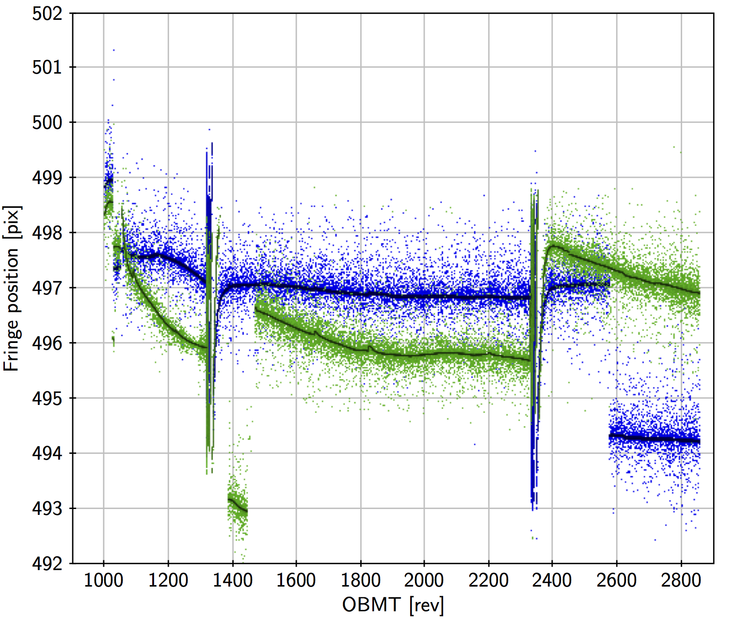
The BAM data show that the basic angle of the Gaia telescopes varies with an amplitude of about 1 mas and a period of 6 hours. The variations are very regular and phased with respect to the direction towards the Sun. For a constant solar aspect angle they are (mainly) a periodic function of the heliotropic spin phase (Figure 3.3).
Generation
During normal operations of Gaia the dedicated BAM CCD is read out once every 23.52 s (approximately). The CCD frame contains the interferograms from both fields of view, so the measurements are strictly simultaneous. The BAM elementary record (one per field of view) contains the estimated AL position (in pixels) of the central fringe, together with the time (OBMT) of the measurement and statistical results from the estimation procedure. The most important statistic is the goodness-of-fit, which is useful for eliminating measurements disturbed by cosmic rays and bright transiting stars.
The BAM data are generated through an off-line analysis of the BAM elementary records using the following inputs:
-
•
the time of each BAM measurement ();
-
•
the corresponding fringe positions in the preceding and following fields, and ;
-
•
the goodness-of-fit measures (weighted RMS fitting errors), and ;
-
•
the heliotropic spin phase ;
-
•
the distance from the Sun to Gaia, .
The first three items are extracted from the BAM elementary records. The times are corrected so that they refer to the mid-time of the CCD exposure. The fringe positions are converted from pixels to angular units as by means of a nominal scale factor ( as). For convenience, and since only the variations of the fringe positions are of interest, constant offsets are subtracted so that and are approximately centred on zero.
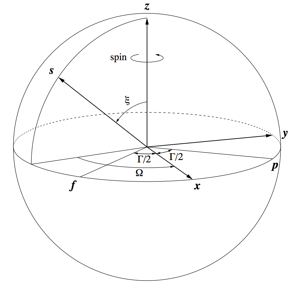
The last two items require information from the attitude and barycentric ephemerides of the Sun and Gaia, and are computed as follows. Using GREM (Section 3.1.5), the distance to the Sun () at the time of the BAM measurement is obtained together with the observed (proper) direction to the Sun, . For the latter, GREM returns the rectangular coordinates in the Centre-of-Mass Reference System (CoMRS) , that is
| (3.31) |
The components of the same vector in the Scanning Reference System (SRS) ,
| (3.32) |
are obtained by the frame rotation (Equation 11 in Lindegren et al. 2012)
| (3.33) |
where is the quaternion representing the attitude of Gaia at the time of the BAM measurement. On the other hand, from Figure 3.3 it is seen that
| (3.34) |
from which and can be computed. (The angles and also appears in the definition of the scanning law of Gaia. However, while the scanning law is defined with respect to a non-physical object called ’the nominal Sun’, the present angles represent the actual physical direction towards the Sun, that is the direction of the energy flux or Poynting vector. The physical and nominal directions may differ by up to about 0.1, which could matter for the description of the basic-angle variations. The angle defined through the equations above may be called the physical heliotropic phase angle in order to distinguish it from the corresponding nominal heliotropic phase angle used in the scanning law.)
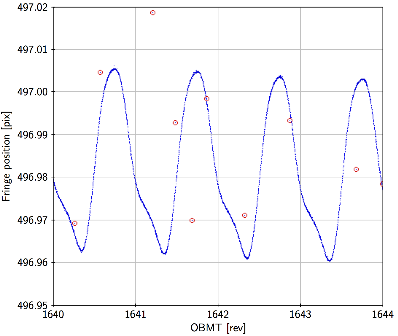
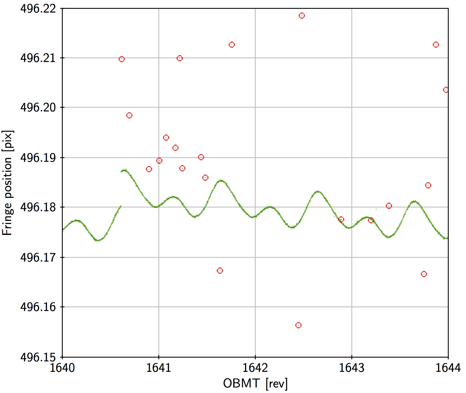
Figure 3.3 shows the fringe position data for a little more than the first year of nominal operations. Major disturbances are caused by decontaminations (affecting OBMT 1316 to 1390 and 2335 to 2400) and telescope refocusing (at OBMT 1443 and 2560). Apart from these, there are long-term variations and a scatter of outliers. Zooming in on a shorter time interval as in Figure 3.6 shows very clearly the 6 hour variations in both fields of view, and also that the outliers affect only a very small fraction of the data.
Jumps such as the one seen in Figure 3.6 at OBMT 1640.6 in the following field of view are relatively common (typically a few per week exceeding 0.1 mas). The jumps sometimes affect only one field of view, sometimes both simultaneously. Detected jumps and their estimated times and amplitudes are an important input to the geometrical calibration model (Section 3.2.5).
The BAM elementary records are processed by fitting simultaneously fitting the jumps and a smooth variation of the fringe positions over a certain interval of time (e.g., between longer data gaps). The generic model (here written for the preceding field, using superscript P) is
| (3.35) |
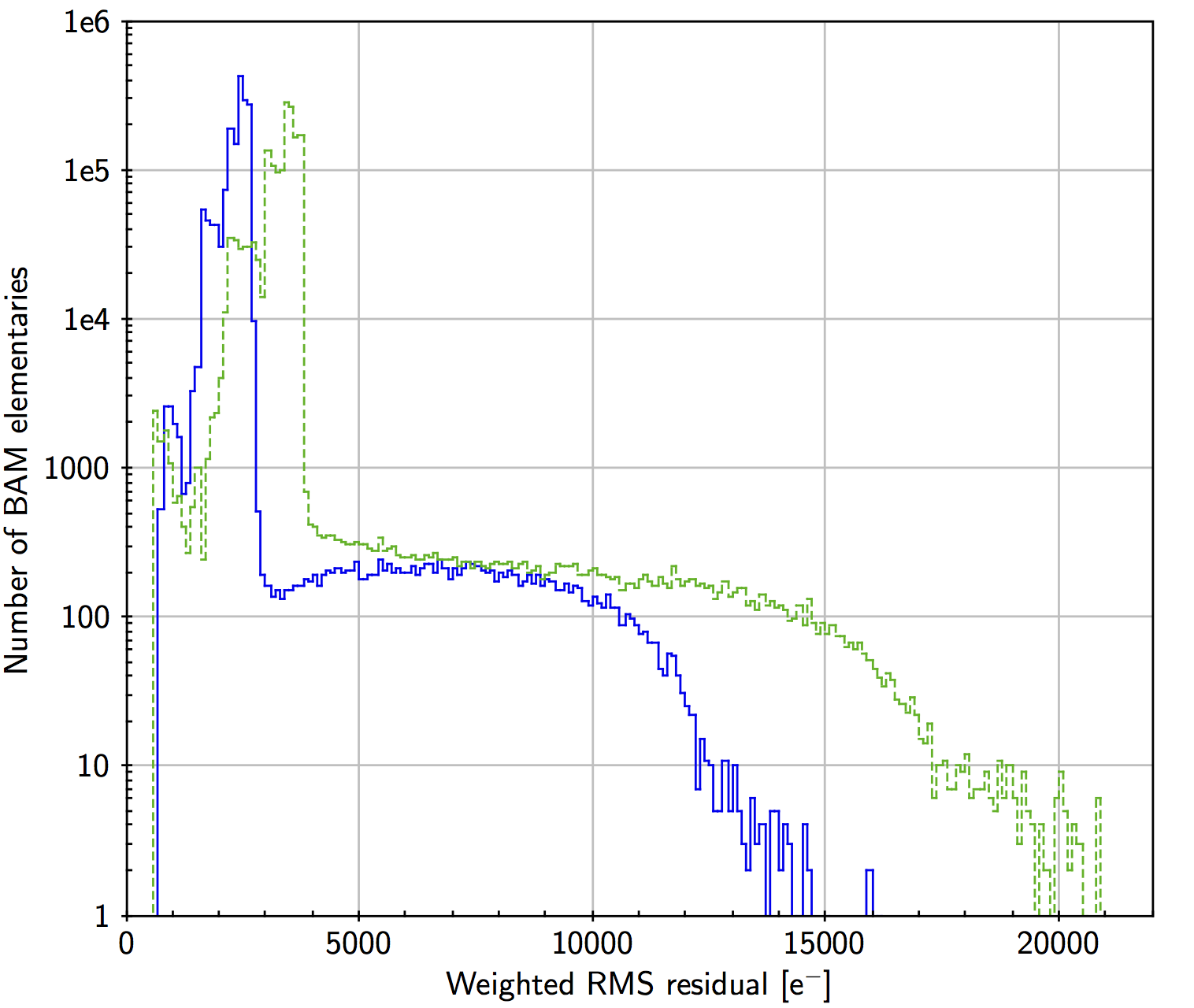
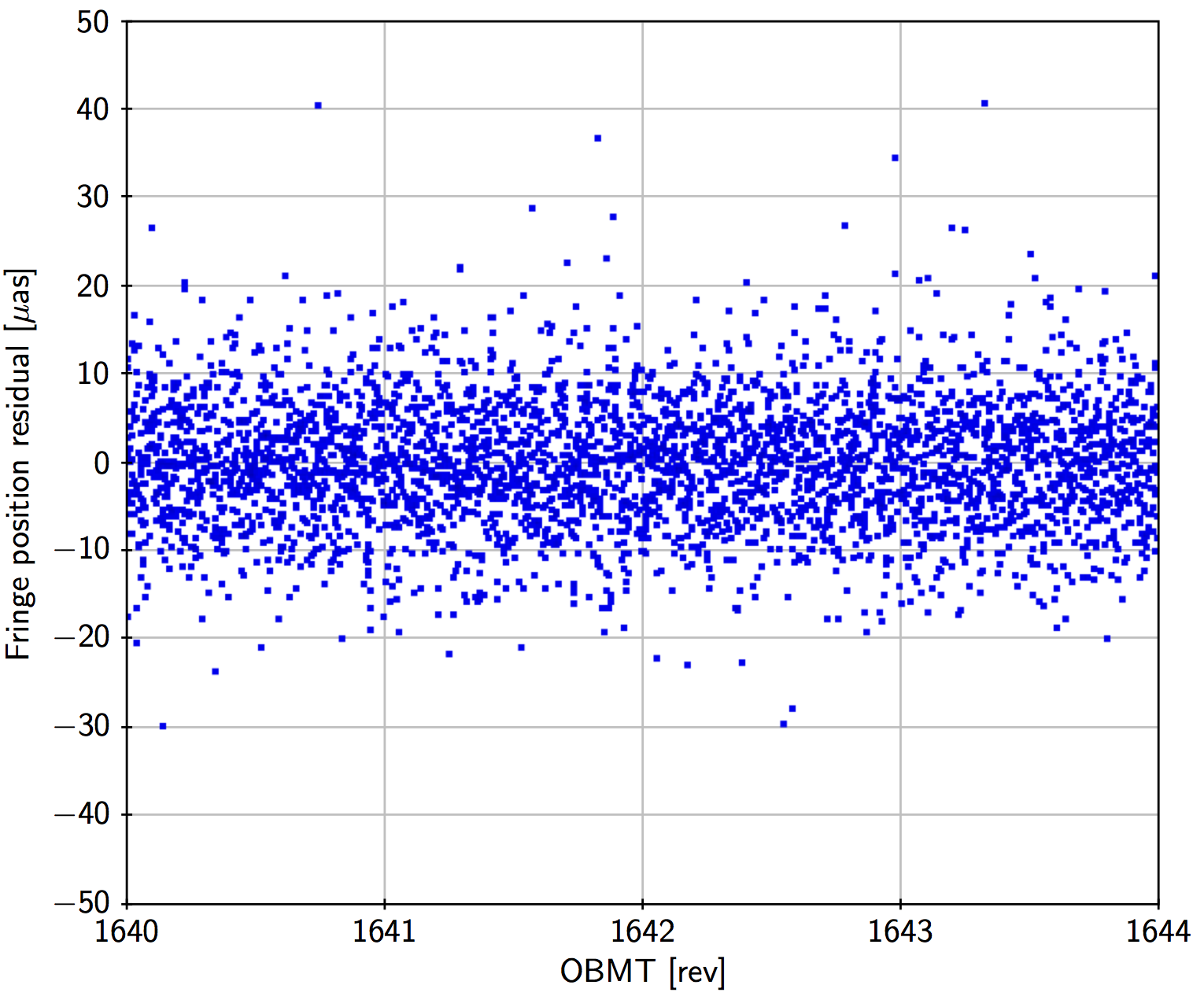
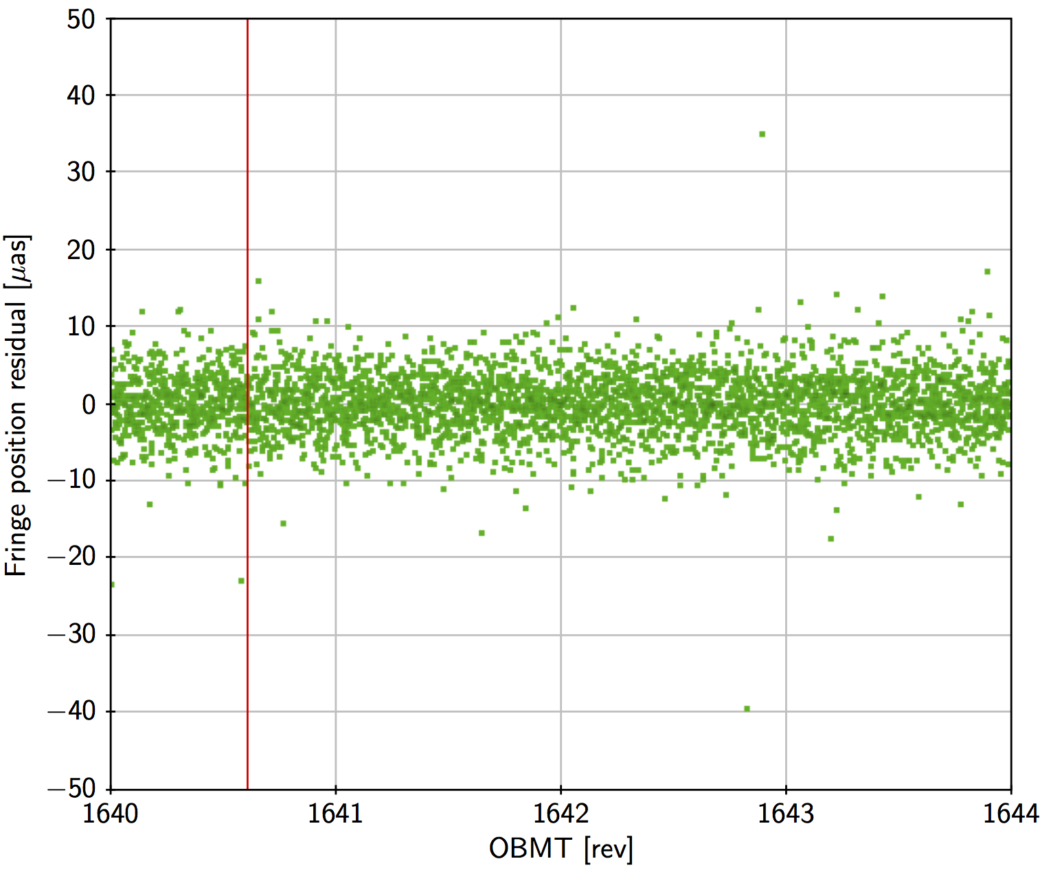
where , are continuous functions of time, represented by cubic splines, and are the times and amplitudes of the jumps. is a ramp function, increasing linearly from 0 to 1 for , where s is the CCD integration time for the BAM data. The width of the ramp sometimes makes it possible to determine the time of the jump to within a few seconds. For example, if the jump occurred exactly halfway through a CCD exposure, it would record a fringe position halfway between the positions recorded immediately before and after the jump. The fitted parameters are , , and the spline coefficients of for and for . Using harmonics was always found to be sufficient to represent the smooth, quasi-periodic variations. The splines use a regular knot sequence with a knot separation of the order of a day (a few times the spin period). A robust fit is made by first removing gross outliers based on the goodness-of-fit statistics , and then iteratively down-weighting isolated points that have large residuals when Equation 3.35 is fitted to the data. Figure 3.7 is an example of the residuals of the fit using a knot interval of 6 hours. With such a short knot interval the residuals usually show no discernible systematics and the RMS residual is about 7 as in the preceding field and 4 as in the following field of view.
The fitted model is strongly non-linear with respect to the times of the jumps, , and the number of jumps, . These are therefore estimated iteratively using a special procedure applied to the residuals of the previous fit, including the jumps detected up to that point. The procedure searches for the time where the tentative insertion of an additional jump would lead to the greatest improvement in the overall fit. If the amplitude of the tentative jump exceeds a fixed threshold, the jump is considered to be significant and added to the list of jumps. This is repeated on until no more significant jump are found.
The model in Equation 3.35 is fitted separately to the BAM measurements in the preceding and following fields of view. The basic angle variation is the difference between the fitted models,
| (3.36) |
Before taking the difference, the jump times are collated between the two fields, so that nearly coinciding times are made to coincide exactly.
The basic-angle correction described above is planned to be used from DR2 (TBC) and onwards. For DR1 a simplified model was used, in which the smooth part of the basic-angle variations is represented by the continuous function
| (3.37) |
The coefficients , , , and were obtained by linear fits to . Although jumps were detected and fitted as described above, they are not included in . Details are given in Appendix A.2 of Lindegren et al. (2016).
Contents
The output of the processing described in Section 3.2.5 consists of a cubic spline function fitted to . A knot interval of about 10 minutes is sufficient to represent the harmonics (up to order ) to better than 0.1 as. Detected jumps are represented by four-fold knots inserted at the appropriate times. A list of detected jumps, , is also produced.
Usage in Gaia processing
The spline function representing the function , including discontinuities at the detected jumps, is used as a first-order correction of all astrometric measurements for the basic-angle variations. Additional corrections are computed in the astrometric solution as part of the geometric instrument model (Section 3.3.5) or global parameters (Section 3.3.6).
The list of detected jumps is used to select suitable breakpoints for the calibration model. Typically, jumps exceeding 0.1 mas (TBC) in amplitude should result in a breakpoint. However, this is not always possible, e.g., if the resulting calibration interval would be too short.