3.3 Calibration models
Author(s): Sergei Klioner
3.3.1 Overview
Author(s): Lennart Lindegren
The astrometric principles for Gaia were outlined already in the Hipparcos Catalogue ESA (1997, Vol. 3, Ch. 23) where, based on the accumulated experience of the Hipparcos mission and the general principle of a global astrometric data analysis was succinctly formulated as the minimization problems (see Lindegren et al. (2012)):
| (3.38) |
Here is the vector of unknowns (parameters) describing the barycentric motions of the ensemble of sources used in the astrometric solution, and is a vector of ‘nuisance parameters’ describing the instrument and other incidental factors which are not of direct interest for the astronomical problem but are nevertheless required for realistic modelling of the data. The observations are represented by the vector which could for example contain the measured detector coordinates of all the stellar images at specific times. is the observation model, e.g., the expected detector coordinates calculated as functions of the astrometric and nuisance parameters. The norm is calculated in a metric defined by the statistics of the data; in practise the minimization will correspond to a weighted least-squares solution with due consideration of robustness issues. The statistical weight of individual observations is composed of a contribution from the formal standard uncertainty of the observation and the excess noise represents modelling errors and should ideally be zero. However, it is unavoidable that some sources do not behave exactly according to the adopted astrometric model (Section 3.3.3), or that the attitude (Section 3.3.4) sometimes cannot be represented by the model used to sufficient accuracy.
The excess noise term is introduced to allow these cases to be handled in a reasonable way, i.e., by effectively reducing the statistical weight of the observations affected. It should be noted that these modelling errors are assumed to affect all the observations of a particular star, or all the observations in a given time interval. (By contrast, the down-weighting factor is intended to take care of isolated outliers, for example due to a cosmic-ray hit in one of the CCD samples.) This is reflected in the way the excess noise is modelled as the sum of two components,
| (3.39) |
where is the excess noise associated with source (if , that is, is an observation of source ), and is the excess attitude noise, being a function of time. For a ‘good’ primary source, we should have , and for a ‘good’ stretch of attitude data we may have . Calibration modelling errors are not explicitly introduced in Equation 3.39, but could be regarded as a more or less constant part of the excess attitude noise. The estimation of is described in Section 3.3.3, and the estimation of in Section 3.3.4.
3.3.2 Aligning the Gaia reference frame
Author(s): Lennart Lindegren
Gaia measures the positions of star images in the focal plane, from which the astrometric solution reconstructs the celestial positions, proper motions, and parallaxes of the sources together with the attitude and calibration parameters. Because the measurements are essentially relative within the field of view, the resulting coordinate system of positions and proper motions is also relative in the sense that its orientation and spin with respect to the celestial reference system (ICRS) are not precisely defined from the measurements themselves. The source and attitude parameters obtained in AGIS are thus expressed in a reference system that is internally consistent and well-defined, but slightly different from ICRS.
The purpose of the frame alignment process is to correct the source and attitude parameters so that they are expressed in a reference system that coincides with ICRS as closely as possible. Gaia observations of extragalactic sources (quasars) are used for this. Quasars are sufficiently distant that their peculiar motions can be neglected; therefore, they define a kinematically non-rotating reference system. Moreover, a subset of the quasars, known as the ICRF, have accurate positions in ICRS determined by radio–interferometric (VLBI) observations. Gaia observations of their optical counterparts allow the origins of and to be aligned with the ICRS.
Section 6.1 in Lindegren et al. (2012) gives the rigorous definition of the rotation correction, then derives a linear approximation applicable to the small corrections that exist in practise. Only the small-angle approximation is described here, as it is sufficient in (nearly) all practical cases and much easier to explain. A similar process was used to align the Hipparcos Catalogue with the extragalactic reference frame (Lindegren et al. 1992).
The ICRS may be represented by the vector triad , where , , and are unit vectors pointing towards , , and , respectively. Since ICRS is non-rotating relative to distant quasars, the directions of these vectors are fixed. The reference system of the source and attitude parameters resulting from the astrometric solution can similarly be represented by a vector triad which deviates slightly from . Moreover, may rotate slowly with respect to . At any particular time the difference between the two systems can be represented by a rotation vector such that
| (3.40) |
The last term indicates that we are in the regime of the small-angle approximation, meaning that terms of the order of can be neglected. If as precision is aimed at, that must consequently be less than about 0.5 . Note that is time-dependent, due to the rotation of , and that it is defined in the sense of a correction to the orientation of .
The astrometric source model (Section 3.3.3) constrains the sources to move uniformly through space, which implies that the time-dependence of must be linear. As long as the correction remains small, it can therefore be written
| (3.41) |
where is the orientation correction at (the reference epoch of the catalogue), and is the spin correction.
The celestial position and proper motion of a source in the ICRS (relative to ) are defined by means of Equation 3.3 and Equation 3.4, where the components of the vectors and are actually the projections of these vectors on . The corresponding source parameters obtained in the astrometric solution, denoted and , are similarly defined by the projections of the same vectors on . It is readily shown that
| (3.42) |
and
| (3.43) |
where , , are the unit vectors introduced in Section 3.3.3. With , , , , , denoting the components of and in , these relations can be written in matrix form as
| (3.44) |
and
| (3.45) |
Given the position and proper motion differences for the same sources expressed in and , these equations can be used to obtain a least-squares estimate of and . The same equations can then be used to correct the source parameters so that they refer to instead of .
The astrometric solution that produced source parameters relative to also produced an attitude estimate in the same reference system. This attitude should also be aligned with if it will be used for the further analysis (e.g., the secondary source update). This is done by applying a time-dependent transformation of the attitude parameters, as described in Section 6.1.3 of Lindegren et al. (2012).
In practise is obtained by comparing the radio positions of ICRF sources ( and in the above equations) with the positions of their optical counterparts as obtained in the astrometric solution (, ). The second version of the ICRF, ICRF2 (Fey et al. 2015) contains at least some 2000 sources that are optically bright enough to be measured by Gaia.
The determination of can use a much larger set of quasars, because Equation 3.45 does not require their precise positions in ICRS to be known, only their proper motions in ICRS (, ). The latter are expected to be very small, but not zero. Apart from various random effects, including the peculiar motions of quasars and optical variability causing centroid displacements (Bachchan et al. 2016), the most important systematic proper motion pattern for quasars is expected to be produced by the secular variation of stellar aberration due to the galactocentric acceleration of the solar-system barycentre (Kopeikin and Makarov 2006). The galactocentric acceleration vector should have a magnitude of m s, pointing more or less towards the galactic centre. The effect on the quasars is an apparent streaming motion towards the galactic centre, described by
| (3.46) |
where and is the speed of light. The magnitude of the effect is thus as. It is not wise to assume that this effect is precisely known; instead the components of in the ICRS should be introduced as additional unknowns when solving for . This leads to an augmented version of Equation 3.45 with six unknowns,
| (3.47) |
If the quasars are reasonably distributed over the celestial sphere, the correlation between the least-squares estimates of and will be small (Bachchan et al. 2016). The additional unknowns will therefore not weaken the solution for , but are essential to eliminate possible biases caused by the acceleration terms.
The orientation, spin, and acceleration parameters represent the lowest-order terms of a general expansion of position and proper motion differences in terms of vector spherical harmonics (Mignard and Klioner 2012). Other terms are expected to be negligible and can be used to check the internal consistency of the Gaia reference frame.
For Gaia DR1, Equation 3.44 was used to align the Gaia reference frame to ICRF at the reference epoch J2015.0, using the optical counterparts of about 2000 sources in ICRF2. However, Equation 3.47 was not used because the short duration of the data (14 months) was insufficient to determine the proper motions of quasars. Instead, it was assumed that the Hipparcos Catalogue was aligned with ICRF at the epoch of the Hipparcos observations (J1991.25). The reference frame of Gaia DR1 was thus aligned with the ICRF at the two epochs J1991.25 and J2015.0, and the proper motion system of Gaia DR1 should then be non-rotating with respect to ICRF to a precision set (mainly) by the alignment of the Hipparcos Catalogue to the ICRF at J1991.25. In this process the effect of the galactocentric acceleration was neglected. Details are given in Section 4.3 of Lindegren et al. (2016).
3.3.3 Astrometric source model
Author(s): Lennart Lindegren
The astrometric model is a recipe for calculating the proper direction to a source () at an arbitrary time of observation () in terms of its astrometric parameters and various auxiliary data, assumed to be known with sufficient accuracy. The auxiliary data include an accurate barycentric ephemeris of the Gaia satellite, , including its coordinate velocity , and ephemerides of all other relevant solar-system bodies. The details of the model have been outlined in Section 3.2 of Lindegren et al. (2012) or Section 3.1.4 and only a short introduction is given here.
As explained in Section 3.1.3, the astrometric parameters refer to the ICRS and the time coordinate used is TCB. The reference epoch is preferably chosen to be near the mid-time of the mission in order to minimize statistical correlations between the position and proper motion parameters.
The transformation between the kinematic and the astrometric parameters is non-trivial (Klioner 2003), mainly as a consequence of the practical need to neglect most of the light-propagation time between the emission of the light at the source () and its reception at Gaia (). This interval is typically many years and its value, and rate of change (which depends on the radial velocity of the source), will in general not be known with sufficient accuracy to allow modelling of the motion of the source directly in terms of its kinematic parameters according to Equation 3.1. The proper motion components , and radial velocity correspond to the ‘apparent’ quantities discussed by in Sect. 8 of Klioner (2003).
The coordinate direction to the source at time is calculated with the same ‘standard model’ as was used for the reduction of the Hipparcos observations (ESA (1997), Vol. 1, Sect. 1.2.8), namely
| (3.48) |
where the angular brackets signify vector length normalization, and is the ‘normal triad’ of the source with respect to the ICRS (Murray 1983). In this triad, is the barycentric coordinate direction to the source at time , , and . The components of these unit vectors in the ICRS are given by the columns of the matrix
| (3.49) |
is the barycentric position of Gaia at the time of observation, and the astronomical unit. is the barycentric time obtained by correcting the time of observation for the Römer delay; to sufficient accuracy it is given by
| (3.50) |
where is the speed of light. See Section 3.2 of Lindegren et al. (2012) for further details.
The iterative updating of the sources is described in Section 5.1 of Lindegren et al. (2012). There the method of identifying potential outliers and estimating the excess source noise is also outlined together with the calculation of the partial derivatives of the coordinate direction with respect to the source parameters.
3.3.4 Attitude model
Author(s): David Hobbs
The Gaia mission allows for astrometric accuracies at the microarcsecond (as) level in stellar positions. To achieve this an accurate determination of the satellite’s attitude is required, including the effects of instantaneous disturbances. The attitude specifies the instantaneous orientation of Gaia in the celestial reference frame, that is, the transformation from the CoMRS defined by to the SRS defined by (see Section 3.1.3) as a function of time. The spacecraft is controlled to follow a scanning law, which for most of the mission will be the Nominal Scanning Law (NSL; de Bruijne et al. (2010)), designed to provide good coverage of the whole celestial sphere while satisfying a number of other requirements. The model used to accurately determine the attitude of Gaia is briefly described in (Section 3.3;Lindegren et al. (2012)).
The attitude model used relies on quaternions (Appendix A; Lindegren et al. (2012)) to model the instrument’s axes expressed directly in the celestial reference frame. Quaternions are an extension of complex numbers (Hamilton 1843) and are commonly used today for spacecraft attitude control, representing spatial rotations in a compact and convenient manner. The instantaneous attitude is represented by a unit quaternion , which has only four components, , satisfying the single constraint . This is easily enforced by normalization.
The attitude quaternion gives the rotation from the CoMRS () to the SRS (). Using quaternions, their relation is defined by the transformation of the coordinates of the arbitrary vector in the two reference systems,
| (3.51) |
In the terminology of (Appendix A.3; Lindegren et al. (2012)) this is a frame rotation of the vector from to . The inverse operation is .
In the attitude processing the components of the quaternions are modelled using B-splines (Appendix B; Lindegren et al. (2012)) giving
| (3.52) |
where () are the coefficients of the B-splines of order defined on the knot sequence . The function is non-zero only for , which is why the sum in (Equation 3.52) only extends over the terms ending with . Here, is the so-called left index of satisfying . The normalization operator guarantees that is a unit quaternion for any in the interval over which the spline is completely defined. Although the coefficients are formally quaternions, they are not of unit length. The attitude parameter vector consists of the components of the whole set of quaternions .
Cubic splines () are currently used in this attitude model. Each component of the quaternion (before the normalization in Equation 3.52) is then a piecewise cubic polynomial with continuous value, first, and second derivative for any ; the third derivative is discontinuous at the knots. When initializing the solution, it is possible to select any desired order of the spline. Using a higher order, such as (quartic) or (quintic), provides improved smoothness but also makes the spline fitting less local, and therefore more prone to undesirable oscillatory behaviour. The flexibility of the spline is in principle only governed by the number of degrees of freedom (that is, in practise, the knot frequency), and is therefore independent of the order. One should therefore not choose a higher order than is warranted by the smoothness of the actual effective attitude, which is difficult to model a priori see Appendix D.4 of Lindegren et al. (2012). Determining the optimal order and knot frequency may in the end only be possible through analysis of the real mission data (see Section 3.3 of Lindegren et al. (2012) for further details).
The iterative updating of the attitude is described in Section 5.2 of Lindegren et al. (2012). There the calculation of the partial derivatives of the coordinate direction with respect to the attitude quaternion are outlined together with the normalization constrains added during the update process to guarantee that the calculated quaternion is always of unit length. This is the final step in the attitude processing and is know as On-Ground Attitude-3 (OGA3).
The excess attitude noise is outlined in Lindegren et al. (2012, Section 5.2.5) and accounts for modelling errors in the attitude representation and could be caused for example by (unmodelled) micro meteoroid impacts, ”clanks” due to sudden redistributions of satellite inertia, propellant sloshing, thruster noise, or mechanical vibrations (Lindegren et al. 2012, Appendix D.4).
Detecting and handling micro-clanks
During early data processing examination of the Gaia attitude rate reconstructed from AF observations reveals numerous irregularities that can be attributed to discrete jumps in the physical AL attitude angle. These jumps are in the following called ‘micro-clanks’. They are seen in both the AL and AC attitude components, but most easily recognised AL thanks to the higher frequency and accuracy of the AL observations.
Micro meteoroid hits cause discontinuities in the physical attitude rate (angular velocity), rather than in the attitude angles, and therefore produce signatures in the data that are distinctly different from those produced by the micro-clanks. Nevertheless, the detection and handling of both effects are sufficiently similar that they can be treated together. In the following we refer to the micrometeoroid hits as ‘micro-hits’, and use ‘micro-events’ as a collective term for micro-clanks and micro-hits.
The existence of micro-clanks was not unexpected — similar effects had been seen in Hipparcos data, and they were explicitly included in the pre-launch Gaia dynamical attitude model (DAM; Risquez et al. (2012)), although their sizes and frequencies were at that time essentially unknown. Based on fairly arbitrary assumptions, the standard 5-year DAM simulation contains some 3100 micro-clanks exceeding 4.4 mas in the AL direction. As will be seen, this is an order of magnitude less frequent than actually observed.
Micro-events can be detected either from the residuals of an astrometric solution, or from rate estimates calculated by numerical differentiation of the field angles derived from successive CCD observations of a source transiting the AF. The latter approach has significant advantages: it does not require a converged astrometric solution (providing an accurate attitude), it is not restricted to the primary sources of the astrometric solution, and it is less sensitive to LSF/PSF calibration errors. It does require a reasonable geometric calibration, which could however be taken from a previous astrometric solution or even from ODAS. It is therefore natural to do the micro-event detection as part of the AGIS pre-processing.
The discontinuities in angle or rate caused by micro-events can in principle be handled by introducing multiple knots at the appropriate times in the spline representation of the attitude quaternion (Appendix A;Lindegren et al. (2012)). A problem that has been left unsolved is how to handle the gated observations in this context. As described by Bastian and Biermann (2005), the effective attitude to be used in the astrometric solution is slightly different depending on which gate is used, and the differences are particularly important when there are rapid variations in rates or angles, as there will be in connection with micro-events. However, once a micro-event has been detected for a certain time, and its amplitude around each axis estimated from the rate data, the specific effects of that event for any gate can be accurately computed from simple models, and does not require any further fitting to the observations. This realisation, and the discovery that micro-clanks are much more numerous than expected, and more easily detected in the rate data than in the residuals of an AGIS solution, motivates a radical change in the strategy for the overall handling of micro-events.
Attitude dead times
Attitude dead time handling is implement in AGIS to avoid periods where large disturbances occur that would render the attitude processing useless. Additionally, if the attitude is completely incorrect in some period this disturbance can cause adjacent regions to also be affected during the iterative updating of the attitude which can in extreme cases cause the entire solution to diverge. The cause of such regions can be many, a few obvious examples are, telescope refocusing, mirror heating to remove contamination, orbital manoeuvres, micro-meteoroid hits, missing or poor observational data, etc. The time span for the dead time can vary significantly from some days, e.g. mirror heating, to a few minutes, e.g. micro-meteoroid hits. As part of the processing, such unstable intervals have been identified manually and the time and duration of the event has been entered into a dead time file which is read when constructing the attitude knot sequence. Dead times are also introduced when no observations are available or when the observations are unmatched in IDT. Gaps are then introduced in the attitude and multiple knots are added at the edge of the gaps with multiplicity equal to the spline order. This allows the spine to be gracefully terminated at the beginning of the gap and restarted after the end of the gap.
3.3.5 Geometric instrument model
Author(s): Lennart Lindegren
The geometric instrument model (or geometric calibration model) is an accurate description of the CCD layout in the Scanning Reference System (SRS; Section 3.1.3) , or equivalently in instrument angles or field angles . The three systems are equivalent because a given direction can be represented in either system by means of the relations
| (3.53) |
where is the field index ( in preceding field of view, in following field of view) and is the conventional basic angle. Conversely, the plane of the SRS and the origin of the along-scan (AL) instrument angle are implicitly defined by the geometric instrument model, or more precisely by certain constraints imposed on the model. The geometrical instrument model is based on the calibration model described in Section 3.4 of Lindegren et al. (2012).
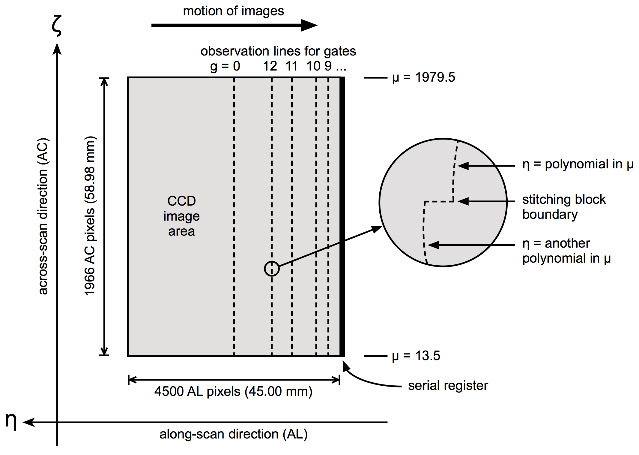
A central concept for the geometric instrument calibration is the observation line, which is an imaginary curve extending over the full width of the CCD image area in the across-scan (AC) direction (Figure 3.8). For ungated observations (gate index ), where all 4500 AL pixels are used to integrate the image, the observation line is nominally situated 2250 TDI lines prior to the serial register (see Table 3.2 for exact numbers). For gated observations using the first gate (), only the last 2900 TDI lines are used for the integration, and the observation line is consequently situated 1450 TDI lines prior to the serial register. The AC pixel coordinate is a continuous variable in the range , with when the image is centrally located in the AC direction of the first pixel column (with the smallest AC field angle ), and when the image is centrally located in the AC direction of the last (1966th) pixel column.
The elementary astrometric measurement, obtained from the transit of a given source over a single (SM or AF) CCD, is the observation time and AC pixel coordinate of the image, . The observation time is calculated, in on-board time, as the read-out time of the reference pixel of the observation window, corrected for the AL offset of the image centroid from the reference pixel, minus the exposure mid-time offset for the relevant (Table 3.2). ( is subsequently converted to TCB using the time ephemeris; see Section 3.1.3.) The observed AC pixel coordinate is obtained by correcting the AC coordinate of the window reference pixel for the AC offset of the image centroid from the reference pixel, but is only available for observations using a two-dimensional window.
The optical design of the Gaia telescopes and the mechanical layout of the focal-plane assembly are such that the TDI lines of all the CCD are very nearly parallel to lines of constant AL field angle in the SRS. (This is a necessary condition for the TDI operation of all the CCDs using the same TDI period.) Thus, to a first approximation the observation lines are short segments of great-circle arcs with a fixed for a given CCD and gate. However, in reality the structure of an observation line is much more complex, as suggested by the ’magnifying glass’ in Figure 3.8. For a given CCD/gate combination, the observation lines are different in the two fields of view, due to the optical distortions being different, and they vary with time due to thermal-mechanical changes in the optics and focal-plane assembly. Additional dependencies (e.g, on window class ) are discussed below.
The observation line for a given combination of field index , CCD index (e.g., in the range 1 through 62 in the AF), gate , and window class is defined in parametric form as
| (3.54) |
The time argument here should be understood as representing the slow variation of the observation lines with time, including for example the basic-angle variations — these are ’slow’ in comparison with the precisions involved in measuring , which are in the s to ms range. The calibration requirements are much stricter AL than AC, and the models for and are separately described hereafter. The particular models described here are the ones used for Gaia DR1 (see Appendix A.1 in Lindegren et al. 2016); more elaborate models will be used for subsequent releases.
The geometric instrument model makes use of shifted Legendre polynomials , where are the usual (non-shifted) Legendre polynomials. The shifted Legendre polynomials are orthogonal on and reach at the end points. The first four polynomials are
| (3.55) |
| TDI lines used | Exposure time | Exposure mid-time offset | |
| 0 | 3,4,7,8,11:4500 | 4494 | 2253.497330 |
| 1 | 3,4 | 2 | 3.500000 |
| 2 | 3,4,7,8 | 4 | 5.500000 |
| 3 | 3,4,7,8,11:14 | 8 | 9.000000 |
| 4 | 3,4,7,8,11:22 | 16 | 13.750000 |
| 5 | 3,4,7,8,11:38 | 32 | 22.125000 |
| 6 | 3,4,7,8,11:70 | 64 | 38.312500 |
| 7 | 3,4,7,8,11:134 | 128 | 70.406250 |
| 8 | 3,4,7,8,11:262 | 256 | 134.453125 |
| 9 | 3,4,7,8,11:518 | 512 | 262.476562 |
| 10 | 3,4,7,8,11:1030 | 1024 | 518.488281 |
| 11 | 3,4,7,8,11:2054 | 2048 | 1030.494141 |
| 12 | 3,4,7,8,11:2906 | 2900 | 1456.495862 |
Notes. is the gate index (0 for un-gated observations, 1–12 for gated observations, with used for the brightest stars). The second column lists the TDI lines used for a given gate, with the TDI lines numbered from 1 to 4500, counted from the serial register. Note that TDI lines 1, 2, 5, 6, 9, and 10 are permanently blocked for light. The exposure time, measured in TDI periods of exactly 0.9828 ms on-board time, is the total number of active TDI lines when a given gate is activated (or none activated if ). The notation 11:4500 means TDI lines 11 through 4500 (inclusive). The exposure mid-time offset is the mean value of the active TDI line numbers, and corresponds to the nominal location of the observation line, expressed as the number of TDI periods before the instant when the pixel content is in the serial register.
AL geometric instrument model
The AL geometric instrument model consists of a nominal part, a constant part, and a time-dependent part:
| (3.56) |
where is the nominal geometry depending on the CCD index and gate, is the constant part depending additionally on the field index and window class, and is the time-dependent part.
The constant part is further decomposed as
| (3.57) |
where the superscripted constants are the calibration parameters and is the normalised AC pixel coordinate. The dependence on CCD gate (’G’) depends on due to the slightly different effective focal lengths in the preceding and following fields of view. The effect of the window class (’W’) also depends on , due to the different PSF/LSF calibration models used for the different window classes and fields. The third term (’B’) in Equation 3.57 represents the intermediate-scale irregularities of the CCD that cannot be modelled by a polynomial over the full AC extent of the CCD. In practise the medium-scale irregularities are largely associated with the discrete stitching blocks resulting from the CCD manufacturing process. The stitching blocks are 250 pixel columns wide, except for the two outermost blocks which are 108 columns wide; the exact block boundaries are therefore , , , , , , . The intermediate-scale errors are modelled by a separate linear polynomial for each stitching block, depending on the block index (where is the floor function, i.e. the largest integer ) and the normalised intra-block pixel coordinate . Here, are the block boundaries given above for . Small-scale irregularities, which vary on a scale of one or a few CCD pixel columns, are not modelled in Gaia DR1 but will likely be included in the improved models used for subsequent releases.
The time-dependent part of the AL calibration needs to take into account the joint dependence on and , which quite generally can be expanded in terms of the products of one-dimensional basis functions. With denoting the normalised time coordinate in calibration interval , we have
| (3.58) |
where is the maximum degree of the polynomial in and is the maximum degree of the polynomial in that is combined with a polynomial in of degree . The current model uses , as for the constant part, and , ; thus Equation 3.58 simplifies to
| (3.59) |
In analogy with Equation (19) in Lindegren et al. (2012), the basic-angle offset can be computed from the calibration parameters as
| (3.60) |
where for the preceding and following field of view, respectively.
| Kind of | Multiplicity | Total | ||||||
| parameter | / | number | ||||||
| 3 | 2 | 62 | 1 | 1 | 1 | 141 | 52 452 | |
| 1 | 2 | 62 | 1 | 1 | 1 | 141 | 17 484 | |
| 3 | 2 | 62 | 9 | 1 | 1 | 1 | 3 348 | |
| 2 | 2 | 62 | 1 | 9 | 1 | 1 | 2 232 | |
| 3 | 2 | 62 | 1 | 1 | 3 | 1 | 1 116 | |
| 3 | 2 | 62 | 1 | 1 | 1 | 87 | 32 364 | |
| 1 | 2 | 62 | 1 | 1 | 1 | 87 | 10 788 | |
| 3 | 2 | 62 | 9 | 1 | 1 | 1 | 3 348 | |
Notes. The columns headed Multiplicity give the number of distinct values for each dependency: polynomial degree (), field index (), CCD index (), gate (), stitching block (), window class (), and time interval ( or ). The last column is the product of multiplicities, equal to the number of calibration parameters of the kind.
AC geometric instrument model
For the AC calibration we have in analogy with Equation 3.56
| (3.61) |
The AC model has fewer breakpoints for the time dependence, no dependence on window class, and no intermediate or small-scale irregularities. Thus,
| (3.62) | ||||
| (3.63) |
where are normalised time coordinates relative to the breakpoints for the AC calibration time intervals.
Summary of calibration parameters
The model as described applies to the 62 CCDs in the astrometric field (AF); for the sky mappers (SM) the nominal calibration , is not updated in the current solution as the SM observations are not used in this release.
Table 3.3 summarises the number of parameters of the different kinds. The total number of calibration parameters is 76 632 for the AL model and 46 500 for the AC model.
Constraints
In order to render all the geometric model parameters uniquely determinable, they must satisfy a number of constraints. Some of them effectively define the origins of the field angles , and hence the SRS, while others are needed to define a unique division between the different components of the model.
The origin of is defined through the constraint
| (3.64) |
Roughly speaking, the mean displacement of the observation lines in the AL direction from their nominal locations should be zero at all times, when averaged over both fields of view and the 62 CCDs of the AF.
The origin of is defined through the constraints
| (3.65) |
Thus, the mean displacement in the AC direction from the nominal locations should be zero at all times, when averaged over the 62 CCDs of the AF. Here, the condition must be separately satisfied in each field of view, in order to define the plane of the SRS.
Additional constraints are needed to ensure a unique division between the the different components of the AL and AC models. These are TBD.
COMA terms
The geometric instrument model only contains terms that depend on the geometry of observation, such as the CCD index, gate, and window class. Formally, it cannot include terms that depend on source parameters such as colour and magnitude; indeed, for consistency the transformation from celestial coordinates to pixel coordinates must be purely geometric.
The image of a point source, as recorded by Gaia, is nevertheless slightly different depend on the colour of the object (e.g., due to wavelength-dependent diffraction effects in the optics) and its magnitude (e.g., due to charge transfer inefficiency in the CCD, which depends on the flux level). These differences will eventually be included in the (colour- and magnitude-dependent) PSF and LSF calibrations, so that the centroid positions obtained by fitting the appropriate PSF/LSFs to the images should be independent of colour and magnitude. Complete elimination of these effects by means of the PSF/LSF calibration will require several iterations of the cyclic processing loop.
In the first few cycles, and especially in the astrometric solution for Gaia DR1, residual colour- and magnitude-dependent effects are therefore expected. For diagnostic purposes it is then useful to add colour- and magnitude-dependent terms, hereafter called COMA terms, in the AL instrument calibration model. In the simplest model the effects are considered to be linear and independent, but different depending on the field of view (), CCD (), and time interval (), in which case the augmented form of Equation 3.56 reads
| (3.66) |
and are the COMA parameters, is a effective wavenumber of source (or the observation of the source), and its magnitude. The reference wavenumber and reference magnitude can in principle be chosen arbitrarily, but for computational reasons they should roughly represent the mean (or median, or mid-range) values of the corresponding quantities. The physical meaning of the reference quantities is that the calculated attitude and (non-COMA part of the) instrument model refer to a source with wavenumber and magnitude .
It is important that the COMA terms are only used internally in AGIS. They are not used, e.g., in the PSF/LSF calibration, where one needs the expected location of an image in the absence of COMA effects, precisely in order to include these effects in the PSF/LSF calibration.
Inclusion of COMA terms in the instrument model for the astrometric solution is however useful for detecting colour- and magnitude-dependent systematics that are not taken care of by the PSF/LSF calibration. They also help to eliminate COMA effects from the computed source, attitude, and geometric calibration parameters, so that they interfere less with the subsequent PSF/LSF calibration. Ideally, and should be insignificant in the final astrometric solution.
3.3.6 Global parameters
Author(s): Sergei Klioner
The astrometric software AGIS can be used to fit arbitrary global parameters, that is, parameters that depend on all or most of the data. A flexible software package in AGIS allows one to fit such parameters in different groups and modes. The primary use of this block is the determination of physical parameters, like the PPN parameter . This will be done in the future data releases. Another application of the global block is to determine instrumental (calibration) parameters characterizing Gaia astrometric instrument as a whole. Examples here are the Velocity and Basic Angle Calibration (VBAC) and Focal Length and Optical Distortion Calibration (FOC). VBAC is intended to determine, to the largest possible extent, Basic Angle variations directly from the astrometric data. FOC determines arbitrary differential distortions of the Gaia astrometric instrument. In Gaia DR1, VBAC was used in the verification of the solution (Lindegren et al. 2016, Appendix E.3). One of the simple variants of VBAC was used for the Gaia DR1 verification and allowed one to determine the coefficients of a Fourier polynomial for the basic angle. Although the fitted coefficients were not used for the released astrometric solution, VBAC has demonstrated that the difference between the fitted coefficients and those determined from the BAM data don’t differ by more than as. This was important to demonstrate the correctness of the BAM measurements. In the future releases both VBAC and FOC will be used to verify and possibly improve the astrometric solutions.
3.3.7 Extended PSF/LSF model
Author(s): Michael Davidson
The cyclic reprocessing environment of IDU allows a more sophisticated LSF/PSF modelling to be performed, relative to the calibration determined in the real-time system (see Section 2.3.2). In this first data release the approach, however, mirrors that used in FL LODC with a few indirect improvements. For example, the bias and background models available in IDU are more complete and have fewer artifacts due to joins between OBMT intervals. The increased processing power available also enables a more flexible solution to be determined (extra spline knots and parameter dependencies).
In future data reductions the main difference with respect to the early LSF/PSF will be the use of a full 2D PSF model, rather than an ALxAC LSF approximation, which is known to limit the performance, particularly when the PSF is asymmetric. This full 2D PSF model will be conceptually similar to the LSF model but it shall use a linear combination of 2D basis functions instead of 1D basis functions. Knowledge of the scene will also permit the full 2D PSF mapping to be extended into the ‘far’ wings, well outside the region sampled by the stellar windows. These diffraction features cause a great number of false detections on-board and so form a valuable data set, along with data from Virtual Objects.
The ultimate aim for the extended LSF/PSF model is to incorporate a Charge Distortion Model (CDM) to handle the effects of Charge Transfer Inefficiency (CTI). The CDM is a very complex problem to solve, and it requires an accurate knowledge of the input signal, so this remains under development. Fortunately the level of radiation damage is significantly lower at this stage of the mission than feared before launch (by a factor of ).