4.5.6 Validation of photometry against known objects
Author(s): Karri Muinonen, Alberto Cellino
Some tests of predicted magnitudes
As mentioned in Section 4.5.3, for some thousands of asteroids the rotation period is known with very good accuracy, based on available ground-based photometric data (light-curves). The celestial coordinates of the spin axis (’asteroid pole’) and a shape have also been computed for many of them, although different investigations carried out by different authors using different computing techniques may have produced a variety of possible pole coordinates, and shape models of different complexity. Available catalogues of asteroid rotation periods and pole coordinates have been exploited to attempt at least a preliminary test of the sparse magnitude measurements obtained by Gaia. To do so, we made use of a modified version of the genetic algorithm developed to invert asteroid Gaia photometry at the end of the mission, when it will be possible to use all the transits recorded for each object to derive a unique solution for the spin (rotation + pole), shape, and mag-phase relation. For sake of keeping to reasonable values the needed CPU time, a simple triaxial ellipsoid shape model is adopted to carry out the photometry inversion computation (Cellino et al. 2009; Santana-Ros et al. 2015).
.
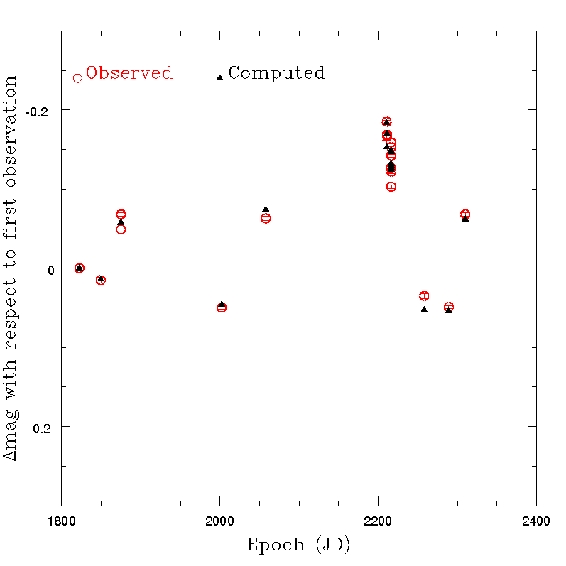
The sparse data present in Gaia DR2 cover only a limited variety of observing circumstances, and are therefore not yet sufficient to run a full inversion algorithm to determine all the unknown parameters, to be compared for validation with currently available knowledge. What is already possible, however, is to run for some objects the inversion program, but with some modifications to treat cases in which the rotation period is already known a priori, as well as the pole coordinates. As for the latter, an uncertainty of 15 degrees in the values published in the literature has been assumed. This is realistic, based on the typical variety of pole solutions published by different authors. In this respect, only the most recent period and poles available in public repositories was chosen for the objects considered in this analysis. The remaining parameters to be determined were the axial ratios of the assumed triaxial ellipsoid shape, the value of the rotation angle at the epoch of the first recorded transit of the object, and the trend of a (nearly linear) magnitude-phase angle variation. In this way, it is possible to compare the time variation of the magnitudes measured by Gaia at different transits with the expected time variation, based on a triaxial ellipsoid shape model applied to the a priori known spin period and pole solution. It is important to note that computations were done in terms of computations of differences of magnitude with respect to the value measured at the epoch of the first recorded transit of each considered object on the Gaia focal plane. In this way, a number of possible systematic effects were automatically removed. It is also important to point out that the computation of the expected magnitudes was carried out by assuming that asteroid surfaces scatter incident sunlight according to a Lommel-Seeliger relation. The analytical computation of Lommel-Seeliger scattering from a triaxial ellipsoid shape has been recently carried out by Muinonen and Lumme (2015); Muinonen et al. (2015) and their results were implemented in our computations.
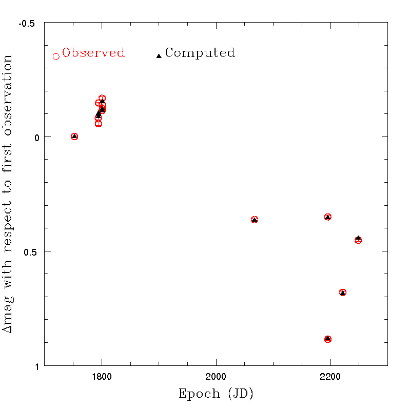
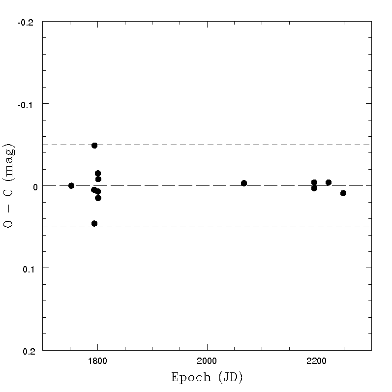
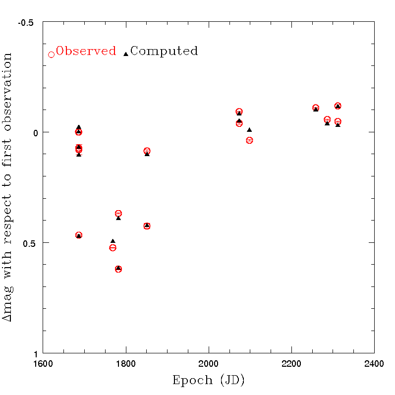
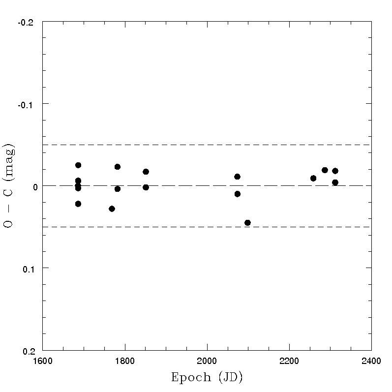
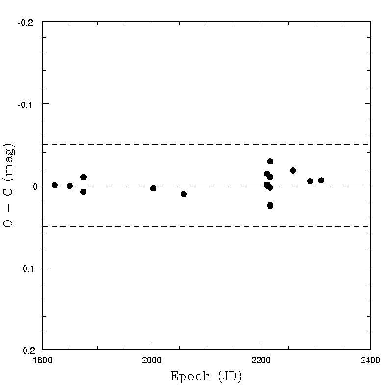
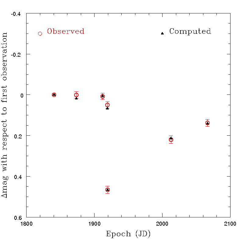
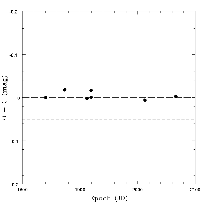
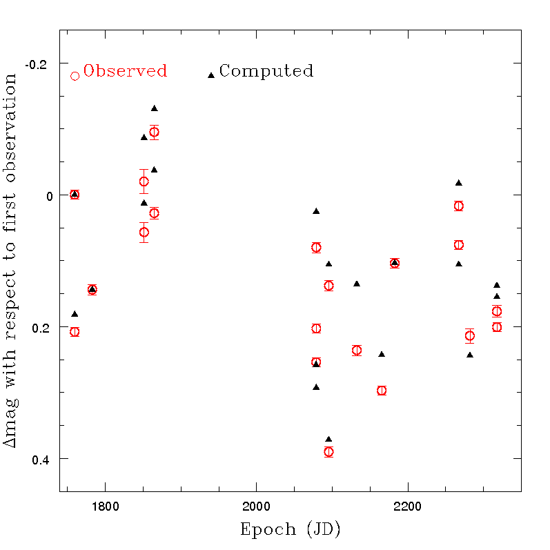
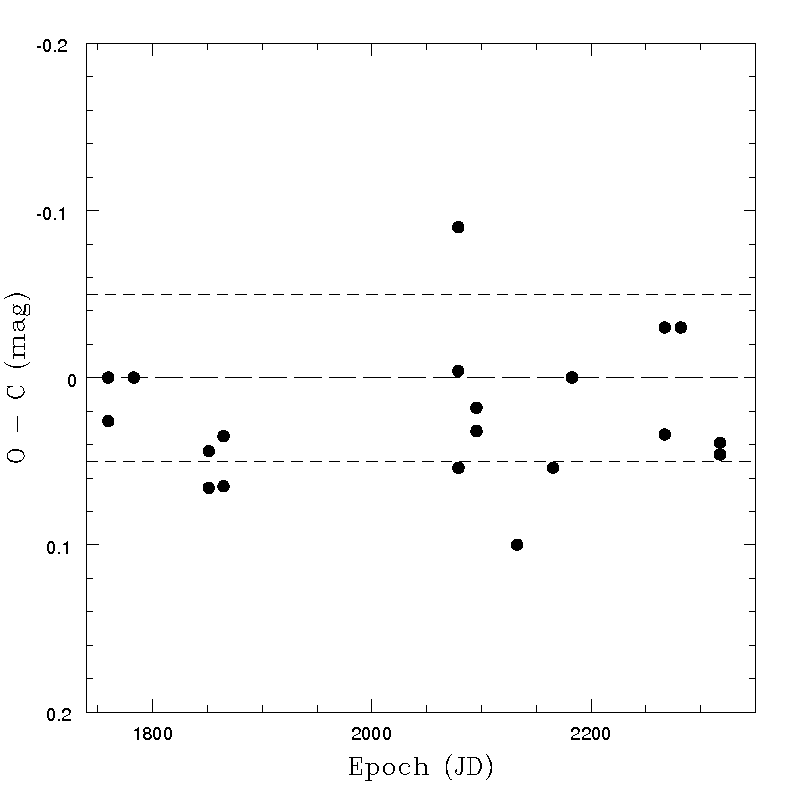
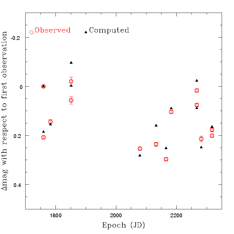
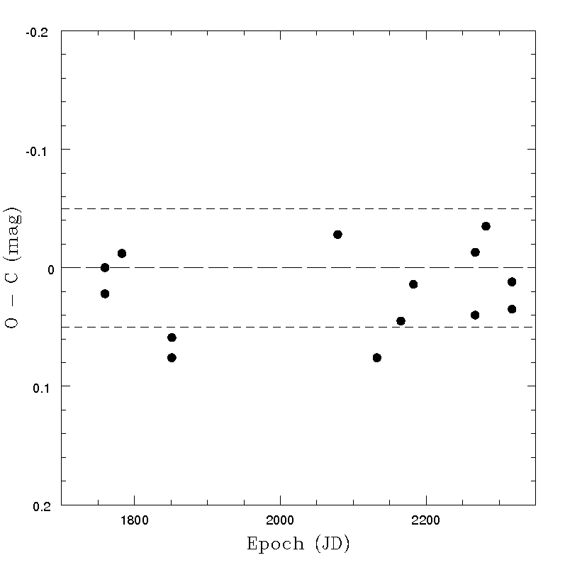
Some examples of the results of this exercise are shown in what follows. Tests were made for a sample of several asteroids, after removing for each object all the transits not satisfying the quality criteria based on nominal error of the derived magnitude and on the colours, as explained in Section 4.5.4. In all cases, a non-spherical shape is responsible of a relevant, periodic photometric variation due to rotation, and the O-C critically depend upon the assumed values of spin period and pole. It should be emphasized that the assumption of an ideal triaxial ellipsoid shape is certainly not very realistic. For this reason, it cannot be expected that the resulting O-C values can turn out to be extremely small, even in the ideal case that the adopted pole coordinates and spin period are perfectly known, and the light scattering behaviour of the objects ideally satisfy the assumed Lommel-Seeliger relatioSome examples of the obtained results in a variety of cases are given in Figure 4.39 - Figure 4.42. The figures show that, generally, the O-C values are below 0.05 magnitudes. Moreover, sudden and striking changes of magnitude, presumably due to shape effects, turn out to be well in agreement with expectations (see, for instance, the case of asteroid (28887) shown in Figure 4.42). This is encouraging, taking into account that the computed magnitudes are based on a simplistic shape model. The overall trend of the variation of the magnitude versus time seems to be in good agreement with the expectations based on available ground-based evidence. Note that the pole coordinates of the computed inversion solutions are allowed to depart by no more than 15 degrees from the values found in the most recent pole computations based on ground-based data. The computed triaxial shapes turned out to be credible, too (though not shown here). It must be understood that even small variations of the solution parameters can produce in most cases (when there are more than just a few available data points) strongly discrepant O-C. Therefore, it seems that the resulting agreement indicates that the observed magnitudes behave as one would expect (and hope) if Gaia photometric data are not affected by large errors and the shapes of the real objects do not depart dramatically from a convex, triaxial ellipsoid approximation.
Note that the Figures displayed in this Subsection show the results obtained for a variety of objects in terms of brightness, taxonomic class, shape and number of available transits after applying the photometry rejection filter defined in Section 4.5.4. Therefore, it seems that the resulting O-C values look quite satisfactory. We note that an analysis was done also in the case of an object, the dwarf-planet (1) Ceres, which is not included in Gaia DR2 due to its excessive brightness and apparent image size which are expected to degrade significantly the quality of Gaia astrometric and photometric results. Ihe resulting magnitudes measured for this object were found to be in very good agreement with expectations. In particular, Ceres has a shape very close to an ideal sphere, and the solution of the photometric inversion computation correctly found a spherical shape, independent, as expected, upon the assumed choice of the spin period and spin axis orientation.
As far as the photometric rejection filter explained in Section 4.5.4 is concerned, it is interesting to note that available tests showed that in several cases using non-filtered magnitudes produces worse fits of the data. A comparison between the results obtained for the O-C computations by using data with or without rejection filter, is shown in Figure 4.43 for the case of asteroid (40) Pomona, an object for which the obtained O-C values are not particularly satisfactory, presumably due to the mentioned limits of a triaxial ellipsoid shape assumption. In this, as in several other cases tested during the data validation procedures, a general improvement of the obtained O-C values was found, if transits not satisfying the photometry rejection filter are discarded.
Summarizing, the results of the exercise described above, though limited to a small sample of objects, suggest that Gaia photometric data for asteroids are in satisfactory agreement with the expectations based on knowledge of the spin properties of the objects when they are available. Moreover, it seems that the photometry rejection filter proposed in Section 4.5.4 tends to improve the results, suggesting that the proposed rejection filter is useful and may play an important role in removing data that are not of a good quality.
Tests on objects observed in situ
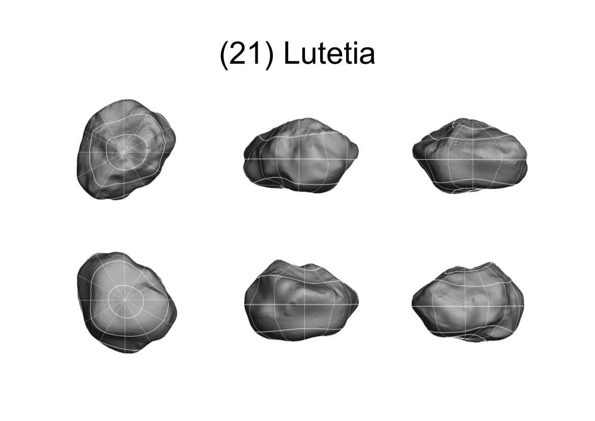
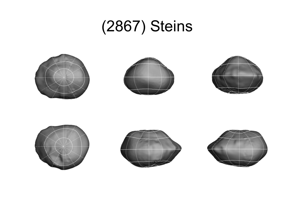
The most compelling criterion of photometry validation consists of comparing the observed Gaia photometric measurements with the expected values computed for known asteroids that have accurately determined rotation periods, pole orientations, and high-resolution shape models. In Gaia DR2, there are only two asteroids that satisfy this criterion: the Rosetta mission flyby asteroids (21) Lutetia and (2867) Šteins. For these asteroids, the Planetary Data System (https://pds.nasa.gov) provides the shape models illustrated in Figure 4.44 as well as the rotation periods and pole orientations described in Table 4.3 (Farnham and Jorda 2013; Jorda et al. 2012; Farnham 2013; Sierks et al. 2011). Furthermore, Table 4.3 gives the phase function parameters and for (21) Lutetia and (2867) Šteins (for the meaning of these parameters, see Muinonen et al. (2010)). In the case of (21) Lutetia, the parameters have been obtained with a linear least-squares procedure described in Muinonen et al. (2010) using the ground-based photometric observations given by Belskaya et al. (2010). For (2867) Šteins, the parameters have been selected on the basis of them being representative of high-albedo E-type asteroids (cf. Muinonen et al. (2010)).
| (21) Lutetia | (2867) Šteins | |
| 8.168270(1) | 6.04681(2) | |
| , | 52.2(4), 7.8(4) | I: 96(5), -85(5) |
| II: 142(5), -83(5) | ||
| 0.40(11) | 0.0 | |
| 0.21(6) | 0.7 |
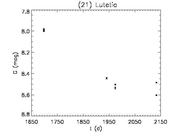
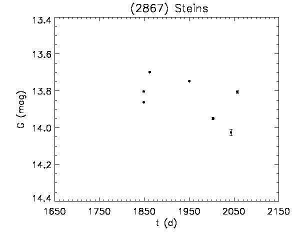
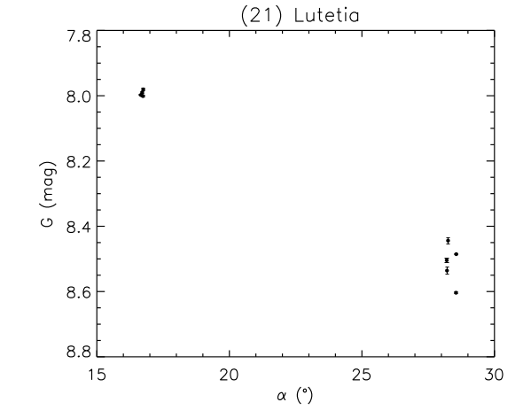
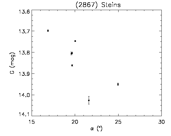
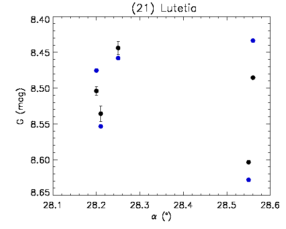
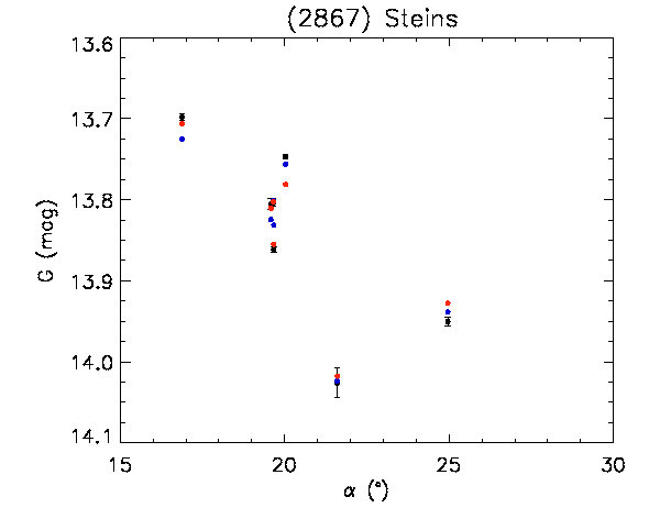
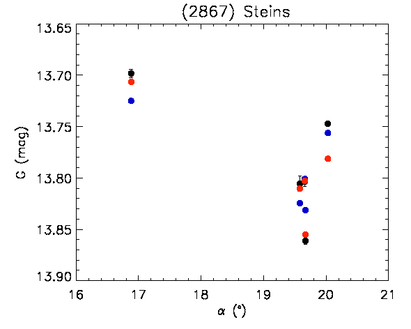
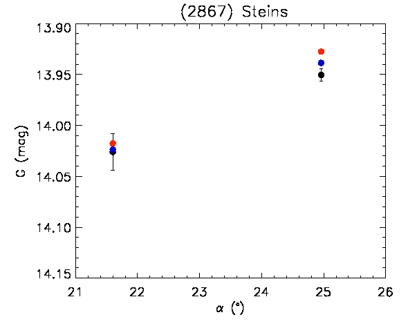
By using the shape models of (21) Lutetia and (2867) Šteins, a study was performed to verify whether it is possible to obtain a convincing validation, although over such an extremely limited sample, of the accuracy of the Gaia SSO photometry. The Gaia DR2 accepted photometric measurements for these two asteroids (after rejecting some data by applying the adopted photometry rejection filter, see Section 4.5.4) are plotted as a function of the epochs of observation, expressed in Julian days, in Figure 4.45. In Figure 4.46, the measurements are plotted as a function of the solar phase angle, expressed in degrees.
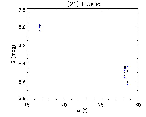
The first study on (21) Lutetia was carried out using a shape model derived from combined ground-based relative photometry and Gaia photometry with convex inversion methods (Muinonen et al. 2018 in preparation, Kaasalainen et al. (2001)). The results showed that the Gaia measurements contributed to the shape modelling with reasonable residuals, with an rms-value of 0.029 mag, corresponding to an rms value of 2.69% for the Gaia flux measurements (see Figure 4.47). At the same time, it was seen that using the best available shape model (Farnham 2013), constructed by combining together a high-resolution shape model based on disk-resolved imaging by Rosetta and a lower-resolution model based on ground-based relative photometry and silhouette observations with adaptive optics, it was not possible to produce a straightforward fit to the Gaia observations. This was interpreted as a strong indication that the Gaia data offers new information on the shape and modifies the currently accepted shape solution.
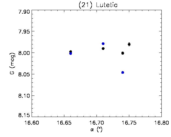
In particular, a closer inspection of the time distribution of the 9 transit magnitudes obtained by Gaia shows that, for 5 of them, the southern hemisphere of the asteroid is predominantly visible. Interestingly, that hemisphere was not mapped by Rosetta and the only constraints on its shape come from ground-based data. It is therefore highly probable that Gaia data provide additional information on that portion of the asteroid surface. In particular, the Gaia photometry with its absolute phase angle dependence relates the size of the southern hemisphere to the size of the northern hemisphere.
An attempt was done to directly model, by using the high-resolution shape, the photometry of the remaining 4 observations, obtained with the northern hemisphere in view. In this case, the high-resolution shape model reproduces the Gaia photometry with a small rms-value of 0.025 mag, corresponding to an rms-value of 2.3 in flux. It is thus possible to conclude that Gaia photometry is probably better than 2%, but the limitations on the shape model accuracy does not allow us to push the analysis further. Also, it is not possible to exclude that some anomalous brightness values are present. Furthermore, the same Lommel-Seeliger scattering model was assumed to be valid everywhere on the surface of Lutetia, and it was also assumed that the phase curve derived from the data by Belskaya et al. (2010) is representative of the entire surface of Lutetia.
The results obtained for (2867) Šteins, whose high-resolution shape model does not suffer from limitations similar to those of (21) Lutetia, strongly support the idea that Gaia photometry is indeed accurate. In the case of this object, there are two pole solutions (see Table 4.3), differing, essentially, only in terms of the zero point of the rotational phase. By directly using the shape model to reproduce the Gaia data, re-sampled at a 5-degree resolution, and by using a Lommel-Seeliger scattering model with a typical E-class asteroid phase function, the rms values of the O-C magnitudes turn out to be 0.018 mag and 0.016 mag (corresponding to rms values of 1.64% and 1.51% for relative flux) for the two pole solutions. Considering the simplicity of the surface scattering modelling utilized, this is a very good if not excellent result depicted in Figure 4.48. Changing the resolution to 3 degrees does not improve the fit further. The remaining limitations, in the case of (2867) Šteins, are still related to details of the shape model, and to some assumptions made on the scattering properties, for instance, when it was derived from the Rosetta images.
In conclusion, the adopted validation procedure appears to show that Gaia epoch photometry, appropriately filtered to eliminate the outliers, has probably an accuracy better than 1-2% in flux, in general. However, given the current limitations on the calibration and processing, we cannot exclude that the sample published in Gaia DR2 might still contain a non-negligible fraction of anomalous data. For this reason, we recommend detailed analysis and careful checks for any applications based on Gaia DR2 photometry of asteroids.