5.4 Processing steps
This section describe in more details the processing steps taken to determine the calibrations and to produce the photometric data included in Gaia DR1.
5.4.1 Pre-processing
Author(s): Francesca De Angeli
The ingestion and pre-processing activities include a number of steps that are necessary for any further processing of the data.
The ingestion phase in particular converts the data as received by the DPC into a data format that is designed and optimized for the photometric processing. This requires matching information contained in different tables using the available cross-match information. Trivial unit conversions are also applied in this stage.
Bias correction and computation of predicted positions are important modules in the pre-processing stage.
Bias correction for the SM and AF observations is taken care within the IDT pre-processing (see Section 2.3.5). Only BP and RP observations need to be corrected for bias in PhotPipe. This is done using the same algorithm and software as the one used in IDT.
Predicted positions of sources at the time of observation are required for the calibration of flux loss and of the geometry of the BP/RP instruments. The computation of predicted positions at the desired accuracy requires the availability of astrophysical coordinates for all sources at a higher accuracy than what is normally available from ground. These were not available yet for this cyclic processing (at the next cycle of operations PhotPipe will start making use of Gaia astrometric results, the accuracy of which will improve at each cycle). For this reason, for Cycle 01 processing no flux loss calibration could be performed. In order to allow the calibration of the geometry of the BP and RP instruments, centroid coordinates were extrapolated from the AF observations onto the BP and RP CCDs to provide a prediction of the location of the source in the window reference system (WRS) at the observation time.
5.4.2 BP/RP processing
Author(s): Giorgia Busso, Francesca De Angeli
The BP/RP processing includes the background calibration and removal, the geometric calibration and its application, the differential dispersion function calibration and the flux and LSF calibration. The differential dispersion function calibration was run for Cycle 01 for validation but results were not applied: only nominal dispersion functions were used convert sample positions into absolute wavelengths. The flux and LSF calibration did not run for Cycle 01. Spectra will be part of future releases as planned within DPAC.
The calibration models have been already defined in section Section 5.3. In this section, more detail will be given on the processing aspects of these calibrations.
Background removal
In the current release only the most dominant contribution to the background is calibrated and then subtracted, that is the one from the stray light. For this, the models described in 5.3.1 are used. If in the maps there are empty bins, interpolation between the neighbours is performed to fill them. The completed map is then used to build a bicubic spline interpolator which, given the heliotropic spin phase and the AC coordinate of the transit to be corrected, computes the background value in electron/pixel/second. This value is converted to the appropriate one, depending on the window sampling (1D or 2D), and then subtracted to the transit to be corrected.
As the calibration for the charge release is not yet available, only the transits with a distance from the charge injection bigger than 50 TDI, are processed at this stage.
Geometric calibration
The differential dispersion function and geometric calibrations are carried out simultaneously. The differential AL geometric and dispersion calibration is determined with respect to an initial fixed arbitrary reference sample position (ARS) and using observations of a sub-sample of the sources selected in a narrow range of colour to ensure that they are of similar spectral types (and their spectra are therefore quite similar).
The calibration proceeds through the following steps:
-
•
Alignment
-
–
Initial estimate of the set of AL position shifts and flux scaling factors to be applied to the observed spectra in a given calibration unit to align them with each other. All the suitable observed spectra are first normalized to a given magnitude (set in the configuration). Within each calibration unit then, all spectra are cross-correlated using a spectrum that is observed at AC position close to the CCD centre (and therefore is representative of an average dispersion) as reference. The result of this process is a set of AL position shift and scaling factor, one per input spectrum.
-
–
Refinement of the set of shifts and scaling factors found in the previous step. This is achieved by fitting a spline to all the observed spectra (after applying the adjustments found in the previous step) in one calibration unit. There will be one spline (reference spectrum) per calibration unit. A correction to the shift and scaling factor first estimates is computed by fitting each of the observed spectra back to the corresponding reference spectrum spline. This is an iterative process where at each iteration a new reference spectrum is computed. The result of this process is a new set of shifts and scaling factors.
-
–
-
•
Differential dispersion calibration In this step the algorithm runs on a set of binned spectra (one per calibration unit) defined using the adjusted spectra obtained from the previous step. Each binned spectrum is computed on a fixed grid, the value of the binned spectrum at each bin is computed as the weighted mean of all observed samples (from all available transits) falling within the bin range. The binned spectra are thus compared to compute a set of additional AL position shifts (one per calibration unit) and a set of corrections for the nominal differential dispersion functions (again one per calibration unit). This is achieved in an iterative process where each iteration consists of two steps:
-
–
a spline is fitted to all the input binned spectra by iteratively adjusting the set of AL position shifts and scaling factors (one per calibration unit);
-
–
an LSQ fit is done with all the input binned spectra and the fitted spline to obtain as a result a set of AL position shifts and corrections for the nominal differential dispersion functions (one per calibration unit).
-
–
-
•
Differential geometric calibration The differential AL geometric calibration is finally derived as the median of the difference between the location of an arbitrary reference sample (ARS) in the observed spectrum (given by the location of the ARS in the reference system adjusted by all the shifts computed so far, the AL position shift per epoch spectrum computed in the alignment and the additional shift per calibration unit computed in the differential dispersion calibration) and the predicted AL data space coordinate for each transit.
It is probably necessary to spend a few more words on the definition of the arbitrary reference sample (ARS). This is the AL location of an arbitrary effective wavelength. For the internal calibration it is irrelevant to know what this wavelength is. The differential AL geometric calibration is defined with respect to the location of the ARS. The application of the geometric calibration determines the observed location of the ARS expressed in pixels within the window.
In future cycles, the location of the ARS will be optimized to make sure that the difference between effective wavelength and nominal wavelength is at its minimum in the vicinity of the ARS for different spectral types. Each sample position corresponds to a given nominal wavelength through the dispersion function. However in general this wavelength is different from the effective wavelength (which is the average wavelength weighted by the spectrum shape and therefore clearly depends on the spectral type). In order to make sure that the chosen ARS is consistent over a large range of spectral types, we need to select a sample position where the difference between the nominal and effective wavelength has a minimum.
For Cycle 01, no optimization was done and the nominal values for reference sample and corresponding wavelength were adopted.
The application is done on all observed spectra. It consists of two steps:
-
•
Differential geometric calibration application: defines for each observed spectrum the AL location of the reference effective wavelength. This is referred to as the observed ARS.
-
•
Differential dispersion calibration application: converts the observed sample AL positions into the pseudo-wavelength system. As mentioned only nominal dispersion functions were used for Cycle 01 processing (and for the generation of the data included in Gaia DR1).
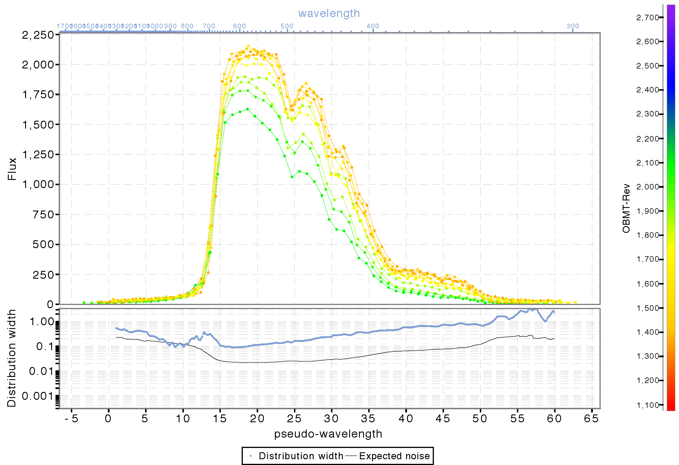
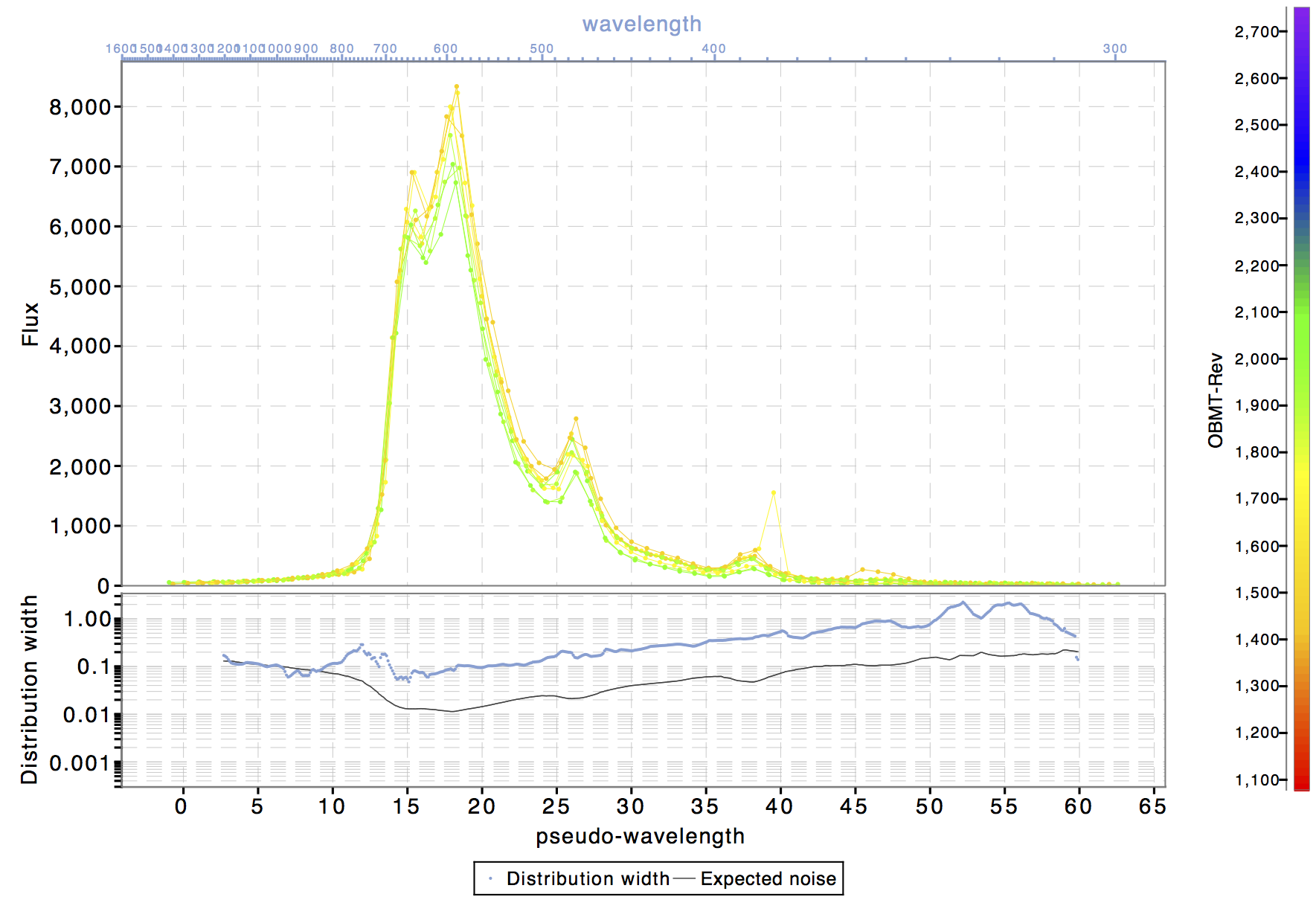
Figure Figure 5.14 and Figure 5.15 show two examples of epoch (BP) spectra for an SPSS source on the left and for an emission line source on the right. Here all epoch spectra have been calibrated for background, differential dispersion and geometry achieving a good alignment of the main features. Clearly no flux and LSF calibration has been applied and contamination effects (varying with time) are quite evident and still present in the spectra. These will be taken care in future cycles.
For Gaia DR1, SSC were computed on epoch spectra calibrated for background, differential dispersion and geometry assuming nominal absolute dispersion. These SSC then gets calibrated within the photometric processing. The photometric results are therefore not affected by the lack of flux and LSF calibration in these first stages into the operations.
5.4.3 Standard star selection
Author(s): Dafydd W. Evans
For Gaia DR1, no standard selection was carried out for the photometric processing of the fluxes. This was because there was no pressing need to reduce the number of transits or sources entering the calibrations and that there were robust procedures, e.g., sigma clipping, within the calibrations to deal with non-constant sources and outliers.
Additionally, at the bright end, due to the small-scale calibration being very complex, it was necessary to maximize the number of transits available entering the calibrations by using all sources. In future data releases, it is intended to use a transit selection procedure to reduce the number of observations used by the calibrations in order to reduce the memory footprint and speed up the iterations.