2.3 Calibration models
Author(s): Claus Fabricius
The calibration models for the sky mapper (SM) and astro field (AF) CCDs must be sufficiently detailed and flexible to allow us to obtain optimal image parameters for astrometry and band photometry, yet not so complex that it becomes unrealistic to carry out the calibrations. The devices are physically almost identical, but, from the way they are operated, they fall in three groups.
The SM CCDs provide large (8012 pixel) images around each source, with the purpose to eventually map the surroundings. The SM CCDs are read in full image mode and with a 22 pixel binning. They have therefore a high readout noise, and are in reality under-sampled. For bright sources ( mag) images will saturate, while for the fainter sources ( mag) a further 22 binning is applied before sending the data to ground. Image parameters for SM will therefore have only little or no weight in astrometry and photometry, but the devices must be calibrated to facilitate their future use.
The first AF CCD, AF1, serves the purpose of confirming the detections from SM, in order to censor detections caused by e.g. cosmic rays. All windows are therefore read with 2D resolution (12 pixel), at the price of a higher readout noise due to the larger number of samples. To save telemetry, the windows sent to ground for fainter sources ( mag) have their samples co-added in each line, and lose again their AC resolution.
The following AF devices, AF2–9, are the workhorses of astrometry and band photometry. They are the CCDs providing the highest potential and therefore the ones with the more demanding requirements.
A limitation of the calibration models in place at the present stage of the mission is that they are focused on the treatment of isolated point sources, and they may not be fully applicable to more complex sources.
2.3.1 Overview
Author(s): Claus Fabricius
Below, we present the more important models applied for the calibration of the SM and AF CCDs. Some are operated on longer timescales and others on shorter scales, but they are all operated on shorter timescales than anticipated before launch. For an overview on the detector performance during the first couple of years in space see Crowley et al. (2016).
The CCD cosmetics (see Section 2.3.4) deal with questions related to individual CCD columns, like saturation level and abnormal response.
The CCD bias and bias non-uniformity (see Section 2.3.5) exposes the difficulties involved in reading CCDs in window mode, where most potential samples are merely flushed. As a consequence, the precise timing for reading a particular column within the short (less than one ms) time available for reading a line of pixels, varies from time to time that column is read, and so does the bias. The model must therefore take the exact readout details into account.
The astrophysical background model (see Section 2.3.3) includes in fact several elements. It must of course describe the complexities of the two sky areas that overlap in the focal plane, but the dominating background source is the stray light which varies strongly with the spin phase of the spacecraft with respect to the Sun, and produces a complex, intermittent pattern on the focal plane. In addition, the background model must also incorporate the charge release trails following the regular charge injections on each CCD (except SM).
The PSF/LSF model (see Section 2.3.2) must encompass many complex effects, but for the first data release, several have been waived. The optical PSF depends on colour, the field of view, and the position in the focal plane, but it also changes with time. On top comes effects induced by the scanning law, by the way the CCDs are operated, and by complex inefficiencies of the charge transfer within the CCDs. A final complexity is that the chromatic image shifts are included in the PSF model as shifts of the PSF origin.
2.3.2 Early PSF/LSF model
Author(s): Michael Davidson, Lennart Lindegren
Two of the key Gaia calibrations are the Line Spread Functions (LSF) and Point Spread Functions (PSF). These are the profiles used to determine the image parameters for each window in a maximum-likelihood estimation (see Section 2.4.8), specifically the along-scan image location (observation time), source flux, plus across-scan location in the case of 2D windows. Of these the observation time is of greatest importance in the astrometric solution, and this is reflected in the higher requirements on the AL locations when compared to the AC locations (Lindegren et al. 2012). Indeed, to increase the signal-to-noise the majority of windows are binned in the across-scan direction and are observed as 1D profiles. A Line Spread Function is thus more useful than a 2D Point Spread Function in these cases. The PSF is often understood as the response of the optical system to a point impulse, however in practise for Gaia it is more useful to include also effects such as the finite pixel size, TDI smearing and charge diffusion. This leads to the concept of the effective PSF as introduced in Anderson and King (2000). Pixelisation and other effects are thereby included directly within the PSF profiles. Calibration of the LSF/PSF is among the most challenging tasks in the overall Gaia data processing, due to the dependence on other calibrations, such as the background and CCD health, and due to uncertainties in crucially measured inputs like colour. This calibration will also become more difficult as radiation damage to the detectors increases through the mission, causing a non-linear distortion. Discussion of these CTI effects can be found in Fabricius et al. (2016). Here we will focus on the LSF/PSF of the astrometric instrument, which in the pre-processing step is assumed to be linear, allowing a more straight-forward modelling and application. The LSF/PSF varies over the relatively wide field of view of each telescope (1.7 by 0.7) and with the spectral energy distribution of an observed source. As previously discussed, the observation time of a source depends on the gate used and, since the LSF/PSF profile can vary along even a single CCD, all gate configurations must be calibrated independently. This can be difficult for the shortest gates due to the relatively low number of observations available. An LSF/PSF library contains a calibration for each combination of telescope, CCD and gate.
Several aspects must be considered when defining a model to represent the LSF/PSF. Firstly, the LSF profiles must be continuous in value and derivative, and they must be non-negative. By definition the full integral in the AL direction is 1, thus neglecting the flux lost above and below the binned AC window. This AC flux loss is calibrated as part of the photometric system. The LSF is normalised as
| (2.11) |
where is the LSF origin. The origin should be chosen to be achromatic (the centroid of a symmetrical LSF is aligned with the origin but this is not true in general), and since image locations are measured relative to it, it should be tied to a physically well-defined celestial direction. However, it is not possible to separate geometric calibration from chromaticity effects within the daily pipeline; this requires the global astrometric solution from the cyclic processing. The origin is therefore fixed as and consequently there will be a colour-dependent bias in this internal LSF calibration. The LSF profile is used to model the expected de-biased photo-electron flux of a single stellar source, including noise, by
| (2.12) |
where , and are the background level, the flux of the source, and the along-scan image location. The index is the along-scan location of the CCD sample under consideration. The actual photo-electron counts will include a random noise component, in addition.
For the practical application, the LSF can be modelled as a linear combination of basis components
| (2.13) |
where basis functions are used. The value of each basis function at coordinate is scaled by a weight appropriate for the given observation. A set of basis functions can be derived through Principal Component Analysis (PCA) of a collection of LSF profiles chosen to represent the actual spread of observations, i.e. covering all devices and a wide range of source colours and smearing rates. An advantage of PCA is that the basis functions are ranked by significance, allowing selection of the minimum number of components required to reach a particular level of residuals. These basis functions can in turn be chosen in a variety of ways; we have used a S-spline model (see Section 2.3.2) with a smooth transition to Lorentzian profiles at the LSF wings. Further optimisation can be achieved to assure the correct normalisation by transforming these bases, although this is beyond the scope of the current document. A set of 51 basis functions were determined from pre-flight simulation data, each represented using 75 coefficients The 20 most significant functions have been found to adequately represent real LSFs, although further improvements are possible.
With a given set of basis functions the task of LSF calibration becomes the determination of the basis weights . These weights depend on the observation parameters including AC position within the CCD, effective wavelength, AC smearing and others. In general, the observation parameters can be written as a vector and the weights thus as . To allow smooth interpolation, each basis weight can be represented as a spline surface where each dimension corresponds to an observation parameter. In the actually implemented calibration system, each dimension can be configured separately with sufficient flexibility to accommodate the actual structure in the weight surface, i.e. via choice of the spline order and knots. In practise, the number of observation parameters has been restricted to two: AC position and effective wavelength (i.e. source colour) for AL LSF, and AC smearing and effective wavelength for the AC LSF. The coefficients of the weight surface are formed from the outer product of two splines with and coefficients respectively. There are therefore weight parameters per basis function which must be fitted.
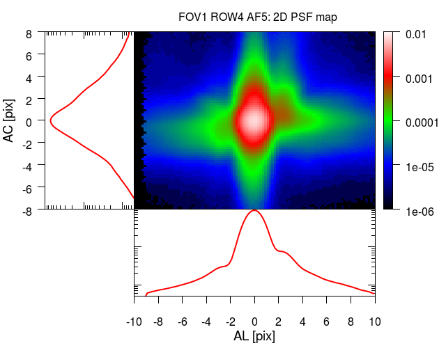
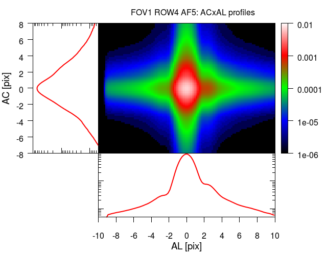
The rectangular telescope apertures in Gaia led to a simple model to approximate the PSF in the daily pipeline. The PSF is formed by the cross product of the AL and AC LSFs. This model has a relatively small number of parameters to fit at the price of being unable to represent all the structure in the PSF. A more sophisticated full 2D model shall be available for the cyclic processing systems (described elsewhere), where there are fewer processing constraints than in the daily pipeline. We have confirmed that the ACAL approximation does not introduce significant bias into the measured observation times for 2D windows. Experiments to compare the fitted observation times using the ACAL versus a full 2D PSF indicate a systematic bias of pixels. An example of the PSF and its reconstruction via the ACAL model is presented in Figure 2.3 and Figure 2.4.
LSF calibrations are obtained by selecting calibrator observations. These are chosen to be healthy (e.g. nominal gate, regular window shape) and not affected by charge injections or rapid charge release. Image parameter and colour estimation for the observation must be successful; good bias and background information must be available. With these data Equation 2.12) can be used to provide an LSF measure per unmasked sample. In the case of 2D windows, the observation is binned in the AL or AC direction as appropriate to give LSF calibrations. The quantity of data available varies with calibration unit. Note that a ‘calibration unit’ in the Gaia pipeline is a given combination of window class (e.g. 1D, 2D), gate, CCD, telescope, possibly time interval (days, weeks, months), and possibly other parameters, e.g. AC coordinate interval on a CCD. For the most common configurations (faint un-gated windows) there are many more eligible observations than can be handled, thus a thinned-out selection of calibrators is used.
A least-squares method is used with the LSF calibrations to fit the basis weight coefficients. The Householder least-squares technique is very useful here as it allows calibrators to be processed in separate time batches and for their solutions to be merged. The merger can also be weighted to enable a running solution to track changes in the LSFs over time (see van Leeuwen 2007). Various automated and manual validations are performed on an updated LSF library before approval is given for it to be used by the daily pipeline for subsequent image parameter determination. There are checks on each solution to ensure that the goodness-of-fit is within the expected range, that the number of degrees-of-freedom is sufficiently positive, and that the reconstructed LSFs are well-behaved over the necessary range of . Individual solutions may be rejected and the corresponding existing ‘best-available’ solution be carried forward. In this way an operational LSF library always has a full complement of solutions for all devices and nominal configurations.
The LSF solutions are updated daily within the real-time system, although they are not approved for use at that frequency. Indeed, a single library generated during commissioning has been used throughout the period covered by this first Gaia data release, in order to provide stability in the system during the early mission. This library has a limited set of dependencies including field-of-view and CCD, but it does not include important parameters such as colour, AC smearing or AC position within a CCD. As such it is essentially a library of mean LSFs and ACAL PSFs. This will change for future Gaia data releases.
S-spline representation of the LSF
This section motivates and defines the special kind of spline functions, here called S-splines, used to represent the cores of the Line Spread Functions (LSFs) via the basis functions (see Section 2.3.2). In some earlier internal documentation the S-splines are called ’bi-quartic’ splines; however, that term should be reserved for two-dimensional quartic splines, and may be particularly confusing in the context of PSF modelling. In Prod’homme et al. (2012) the S-spline is referred to as a special quartic spline.
A physically realistic model of the LSF should satisfy a number of constraints, including non-negativity () and that it is everywhere continuous in value and derivative. Since diffraction is involved, one can also expect that spatial frequencies above are negligible, where m is the along-scan size of the entrance pupil and nm the short-wavelength cut-off. The effective LSF, which includes pixelisation (Section 2.3.2), should in addition satisfy the shift-sum invariance condition,
| (2.14) |
where is the pixel size. This condition immediately follows from the conservation of energy: the intensity of the image corresponds to the total number of photons, independent of the precise location of the image with respect to the pixel boundaries. Numerical experiments indicate that the fitted LSF model should be shift-sum invariant in order to avoid estimation biases as function of sub-pixel position.
A cubic spline is a piecewise polynomial function that is continuous in value and first two derivatives. It is naturally smooth, and therefore to some degree band-limited, and the non-negativity constraint can be enforced by the fitting procedure. A cubic spline defined on a regular knot sequence with knot separation is, moreover, strictly shift-sum invariant, and would thus appear to be ideal for the LSF modelling. Unfortunately, it turns out that a cubic spline with knot separation is not always flexible enough to represent the core of the LSF for Gaia. The basic reason for this is that the optical images in Gaia are under sampled by the CCDs: , while the sampling theorem requires . Increasing the order of the spline does not help: it makes the spline smoother, but not more flexible.
To obtain greater flexibility it is necessary to decrease the knot interval, but then the shift-invariance condition is in general not satisfied. However, among the splines that use a fixed knot interval (for integer ), there exists a subset of splines that do respect the shift-sum condition. These are the S-splines. The simplest way to construct an S-spline is to take an ordinary spline of order , defined on a regular knot sequence with knot interval , and convolve it with a rectangular (boxcar) function of width . It is readily seen that the result is a spline of order , with the same knot interval as the original spline, but respecting the shift–sum invariance. Since the original spline can be expressed as a linear combination of B-splines (splines with minimal support), the S-spline can be expressed as a linear combination of B-splines convolved with the rectangular function.
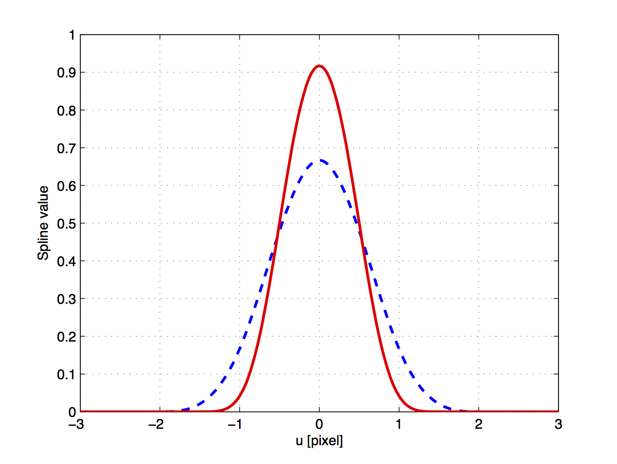
The S-splines used to represent the cores of the basis functions , and hence of , were obtained with and . They are thus quartic splines defined of a regular knot sequence with knot separation , and can be written as a linear combination of the functions , where
| (2.15) |
for . Alternatively, can be obtained by adding two adjacent quartic B-splines. Figure 2.5 shows this function together with the cubic B-spline for knot interval . Although both functions satisfy Equation 2.14, the S-spline can clearly represent peaks of the LSF that are narrower than is possible with the B-spline. Other choices than and are possible but have not been tested.
While the decomposition of a given spline in terms of B-splines is always unique, the decomposition in terms of is not necessarily unique. This is not a problem as long as the coefficients of are not directly used to parametrise the LSF, but are only used to represent pre-defined basis functions such as . When fitting an S-spline to the possible non-uniqueness of the coefficients can be handled by using the pseudo-inverse.
2.3.3 Astrophysical background
Author(s): Nigel Hambly
The astrophysical background incident on the focal plane of Gaia is dominated by stray light (Mignard 2014), in part because the compact and folded design (Safa et al. 2004) of the various optical instruments leaves very little opportunity for stray light path baffling. The lower rows (1–4) of the focal plane have a diffuse background signal that is dominated by sunlight scattered around the DSA while in the higher rows (5, 6 and 7) it is the diffuse optical background from the Milky Way that dominates. Hence the background consists of a high amplitude, rapidly changing photoelectric component that repeats on the satellite spin period. Furthermore, this component evolves slowly in both amplitude with the L2 elliptical orbital solar distance and in phase as the scanning attitude changes with respect to the Ecliptic and Galactic planes. Superposed on this are transient spikes in background due to very bright stars and bright Solar system objects transiting across or near the focal plane. Moreover, there are two non-photoelectric components to the background signal. These are a charge release signal associated with artificial charge injections which are used for on-board radiation damage mitigation (Prod’homme et al. 2011) and the dark current signal. The photoelectric background signal varies routinely over three orders of magnitude depending on instrument and spin phase with values as low as and up to electrons per pixel per second. Regarding the non-photoelectric signals, the charge release signal currently varies between 1 and 10 electrons per pixel per second in the first TDI line immediately after the last injection line but rapidly diminishing to 1% of this level after the following TDI lines, while the dark signal is all but negligible (see Section 2.3.4).
The parametric model for the astrophysical background consists of the outer product of two one-dimensional spline functions (van Leeuwen 2007) which defines a flexible two-dimensional surface model known colloquially as a ‘bispline’. In the along-scan direction the spline function is quadratic with knots evenly spaced at intervals that adapt to the available data density. In regions of high density that generally exhibit higher background fluctuations on smaller spatial scales, and in which there is a higher density of data to constrain the model, knots are more closely spaced. Typically the along-scan knot interval is in the range 1 to 10 arcminutes. In the across-scan direction the spline function is linear, allowing for sudden discontinuities in the gradient of the stray light pattern. Knot positions are placed at fixed, unevenly spaced positions to best follow rapid changes in the stray light pattern in the across-scan direction. The charge release model consists of a simple empirical look-up table (LUT) as a function of TDI line index following the last charge injection line with a power-law scaling as a function of that injection level present at the same column position on the CCD. This enables a single charge release LUT calibration per device when applied in conjunction with the across-scan profile of the charge injection for the same device which is also characterised via a LUT.
2.3.4 CCD cosmetics
Author(s): Michael Davidson
The focal plane of Gaia contains 106 CCDs each with 4494 lines and 1966 light-sensitive columns, leading to it being called the ‘billion pixel camera’. The pre-processing requires calibrations for the majority of these CCDs, including SM, AF and BP/RP, in order to model each window during image parameter determination. Where effects cannot be adequately modelled, the affected CCD samples can be masked and the observations flagged accordingly. The CCDs are affected by the kind of issues familiar from other instruments such as dark current, pixel non-uniformity, non-linearity and saturation (see Janesick 2001). However, due to the operating principles used by Gaia such as TDI, gating and source windowing, the standard calibration techniques need sometimes to be adapted. The use of gating generally demands multiple calibrations of an effect for each CCD. In essence each of the gate configurations must be calibrated as a separate instrument.
An extensive characterisation of the CCDs was performed on ground, and these calibrations have been used in the initial processing. The effects must be monitored and the calibrations redetermined on an on-going basis to identify changes, for instance the appearance of new defects such as hot columns. To minimise disruption of normal spacecraft operations, most of the calibrations must be determined from routine science observations. Only a few calibrations demand a special mode of operation, such as ‘offset non-uniformities’ and serial-CTI measurement (see Section 2.3.5 and Fabricius et al. (2016)). There are two main data streams used in this calibration: 2D science windows and Virtual Objects (VOs). The 2D science windows typically contain bright stars, although a small fraction of faint stars which would otherwise be assigned a 1D window are acquired as 2D (known as Calibration Faint Stars). VOs are ‘empty’ windows which are interleaved with the detected objects, when on-board resources permit. By design the VOs are placed according to a fixed repeating pattern which covers all light-sensitive columns every two hours, ensuring a steady stream of information on the CCD health. The VOs allow monitoring of the faint end of the CCD response while the 2D science windows allow us to probe the bright end.
The dark signal (or dark current) is the charge produced by each column of a CCD when it is in complete darkness. While such condition was achieved during the on-ground testing it is not possible to replicate in flight as there are no shutters on Gaia. The observed VO and science windows must therefore be used to determine the dark signal for each gate setting, although these also contain background, source and contamination signal, bias non-uniformity and CTI effects. A sliding window of 50 revolutions is used to select eligible input observations, for instance those not containing multiple gates or charge injections. The electronic bias (including non-uniformity) is subtracted from each window and a source mask is created via an N-sigma clipping of the de-biased samples. The leading samples in the window are also masked to mitigate CTI effects. A least-squares method is then used to estimate a local background for the window (assumed to be uniform), and this in turn can be subtracted to provide a measure of the dark signal in each CCD column covered by the window. In this manner measures can be accumulated for each column over the 50 revolution interval, and then a median taken to provide a robust dark signal value.
In an ideal device there would be a linear response between the accumulated charge and the output of the Analogue-to-Digital Converters (ADCs) at all signal levels. In reality the response typically becomes non-linear at high input signals for a variety of reasons (see Janesick 2001). Although the linearity has been measured before launch, a calibration has not yet been implemented in the daily pipeline due to the uncertainty in determination of the input signals, which require detailed knowledge of a range of coupled CCD effects. In the meantime a conservative linearity threshold has been used to allow masking of samples which may be within the non-linear regime. A related topic is the pixel non-uniformity which represents the variation in sensitivity across the CCD. In Gaia we observe only the integrated sensitivity of the pixels within a particular gate so this is known as the Column Response Non-Uniformity. Similarly no in-flight calibration has yet been performed apart from the extreme case to identify ‘dead’ columns. These are columns which appear to have zero sensitivity to illumination and can be found using bright-star windows. The accumulated samples for a dead column have a distribution which is consistent with the expected dark signal plus read out noise. The CCDs used on Gaia have been selected for their excellent cosmetic quality.
At the highest signal levels various saturation effects occur on the device and within the ADC. There can be very large differences in the effective saturation level across a single device, or even between neighbouring columns, for example due to variation in the Full Well Capacity. For reasons beyond the scope of this paper the saturation level can oscillate or jump depending on the read-out sequencing. An algorithm has been developed to measure the lowest observed saturation level for each gate and column to allow conservative masking of samples. A Mexican hat filter is applied to the accumulation of samples from bright-star windows to identify over-densities of data at particular signal levels, using analytical significance thresholds. The lowest significant peak is then taken as the saturation level. If no peak is found then the maximum observed sample for that column is used.
The calibrations discussed above are computed daily in the framework of the First-Look system (see Section 2.5.2) and, if they are judged to be satisfactory, the corresponding software libraries are subsequently used in the pipeline.
2.3.5 CCD bias and bias non-uniformity
Author(s): Nigel Hambly
As is usual in imaging systems that employ charge-coupled devices (CCDs) and analogue-to-digital converters (ADCs) the input to the initial amplification stage of the latter is offset by a small constant voltage to prevent thermal noise at low signal levels from causing wrap-around across zero digitised units. The Gaia CCDs and associated electronic controllers and amplifiers are described in detail in Kohley et al. (2012). The readout registers of each Gaia CCD incorporate 14 prescan pixels (i.e. those having no corresponding columns of pixels in the main light-sensitive array). These enable monitoring of the prescan levels, and the video chain noise fluctuations for zero photoelectric signal, at a configurable frequency and for configurable across-scan (AC) hardware sampling. In practise, the acquisition of prescan data is limited to the standard un-binned (1 pixel AC) and fully binned (2, 10 or 12 pixel AC depending on instrument and mode) and to a burst of 1024 one millisecond samples each once every 70 minutes in order that the volume of prescan data handled on board and telemetred to the ground does not impact significantly on the science data telemetry budget.
Video chain offset levels and total detection noise
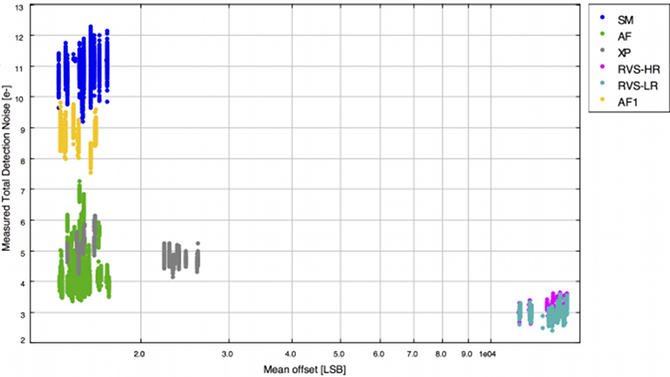
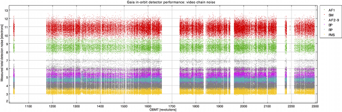
The read noise (or more correctly the video chain total detection noise including noise contributions from CCD readout noise, ADC and quantisation noise etc.) can be assessed from the short timescale fluctuations measured in the prescan levels. Figure 2.6 shows the offset levels and measured total detection noise for the FPA science devices. Table 2.5 gives a summary of the required and measured noise properties of the various instrument video chains. From the sample-to-sample fluctuations measured in the 1 sec prescan bursts, all devices are operating well within the requirements.
We find that all devices are operating nominally as regards their offset and read noise properties.
| Instrument | Mean gain | Total detection noise per sample | ||
| and mode | LSB / e | Required / e | Measured / e | Measured / LSB |
| SM | 0.2569 | 13.0 | 2.783 | |
| AF1 | 0.2583 | 10.0 | 2.249 | |
| AF2–9 | 0.2578 | 6.5 | 1.113 | |
| BP | 0.2464 | 6.5 | 1.273 | |
| RP | 0.2484 | 6.5 | 1.165 | |
| RVS–HR | 1.7700 | 6.0 | 5.779 | |
| RVS–LR | 1.8185 | 4.0 | 5.394 | |
Offset stability
The approximately hourly monitoring of the prescans is suitable for characterising any longer timescale drifts in the offsets characteristics. For example in Figure 2.7 we show the total video chain detection noise as measured from prescan fluctuations over an extended period of over 1000 revolutions (corresponding to more than 250 days). Over this period (July 2014 to May 2015) there is no discernible degradation in the video chain performance.
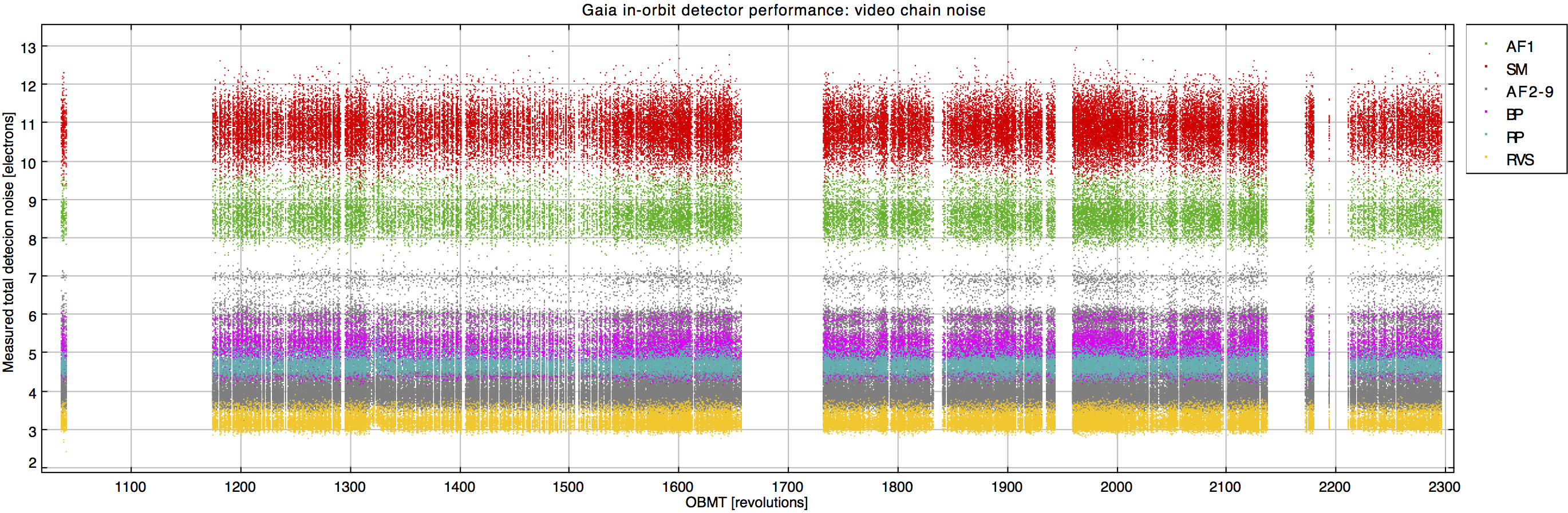
In Figure 2.8 we show the long timescale stability of one device in the Gaia focal plane. In this case (device AF2 on row 4 of the FPA) the long term drift over more than 100 days is ADU apart from the electronic disturbance near OBMT revolution 1320 (this was caused by payload module heaters being activated during a ‘de-contamination’ period in September 2014). The hourly monitoring of the offsets via the prescan data allows the calibration of the additive signal bias early in the daily processing chain including the effects of long timescale drift and any electronic disturbances of the kind illustrated in Figure 2.8. The ground segment receives the bursts of prescan data for all devices and distils into ‘bias records’ one or more bursts per device the robustly estimated mean levels along with dispersion statistics for noise performance monitoring. Spline interpolation amongst these values is used to provide an offset model at arbitrary times within a processing period. Figure 2.9 shows a detailed example around the large excursion seen in Figure 2.8.
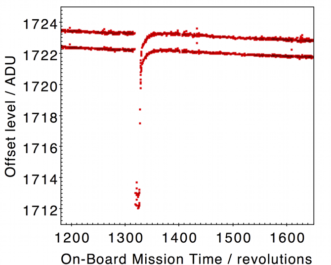
Figure 2.8 illustrates the small offset difference between the un-binned and fully binned sample modes for the device in question. In fact there are various subtle features in the behaviour of the offsets for each Gaia CCD associated with the operational mode and electronic environment. These manifest themselves as small (typically a few ADU for non-RVS video chains, but up to 100 ADU in the worst case RVS devices), very short timescale (10 s) perturbations to the otherwise highly stable offsets. The features are known collectively as ‘offset non-uniformities’ and because the effect presumably originates somewhere in the CCD–PEM coupling it is also known as the ‘PEM–CCD offset anomaly’. The effect requires a separate calibration process and a correction procedure that involves the on-ground reconstruction of the readout timing of every sample read by the CCDs since they are a complex function of the sample readout sequencing. This procedure is beyond the time-limited resources of the near real-time daily processing chain and is left to the offline cyclic data reductions at the Data Processing Centres associated with each of the three main Gaia instruments. However the time-independent constant offset component, resulting from the prescan samples themselves being affected and yielding a baseline shift between the prescan and image-section offset levels, is corrected. This baseline offset correction to the gross electronic bias level of 1400 to 2600 ADU varies in size from ADU to ADU amongst the SM, AF, BP and RP devices. The remaining readout timing-dependent offset non-uniformities are not corrected for in Gaia DR1 but they will be corrected in offline reprocessing for subsequent data releases.