5 Photometry 5.2 Properties of the input data 5.4 Processing steps

5.3 Calibration models

5.3.1 BP/RP background model

Author(s): Giorgia Busso

The astrophysical background signal on the Gaia CCDs has at least three components, of different origin:

1.

the ”canonical” diffuse astrophysical background and the stray light, caused by light falling on the focal plane;
2.

two components, related to the CCD electronics, i.e. the dark current signal (dealt with separately) and the charge release;
3.

the stray light has the biggest contribution to the background signal and dominates the other components.

The background model takes into account only the stray light.

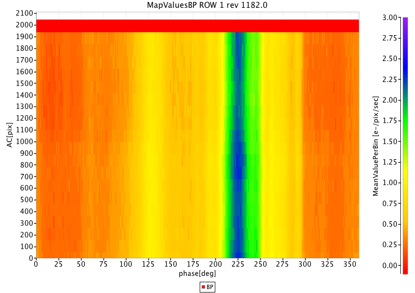
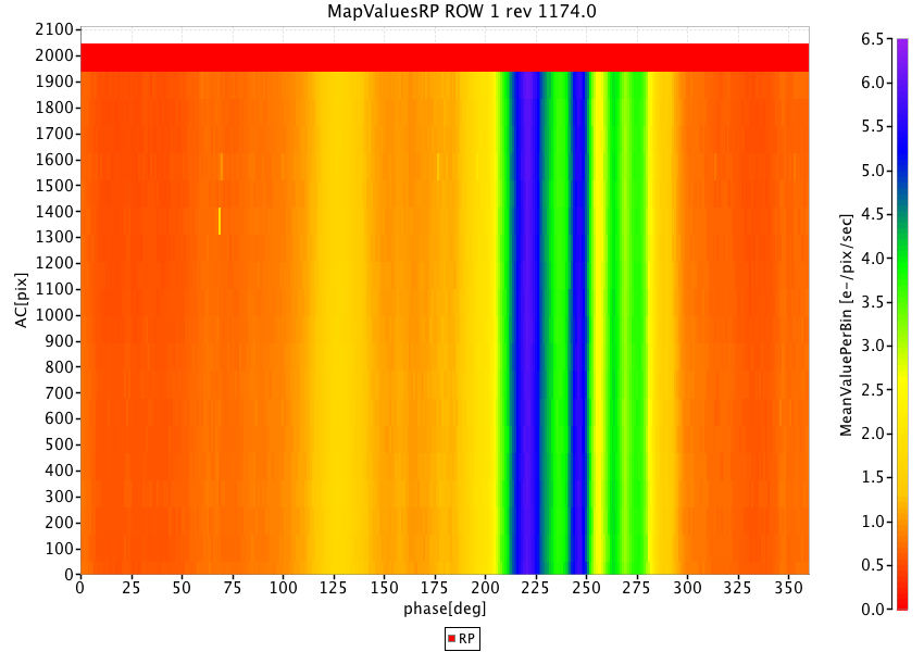
The majority of the stray light is caused by the Sun and the strength of this effect depends on the position of the Sun with respect to the satellite. It shows a periodicity corresponding to the satellite spin phase and a slow evolution in amplitude with the orbital solar distance. Other contributions are in phase with the scanning law, showing contributions from the Ecliptic and Galactic planes.

As a model we used a discrete map, obtained by accumulating two days of observations (Virtual Objects, i.e. empty windows acquired for calibration purposes) with distance from the charge injection higher than 50 TDI lines (to avoid the charge release component). For every transit, the median value on all samples is computed, to avoid the accidental contribution of cosmic rays, and also the AC coordinate and the heliotropic spin phase (Figure 3.3) are calculated. The map is built on a grid of 360 bins in the spin direction (one bin is 1 degree) and 20 bins in the AC direction (one bin is $\sim$ 200 pixels, corresponding to $\sim$ 35 arcsec). All the transits belonging to the same bin are averaged to obtain a median value, to remove outliers. Examples of stray light maps are shown in Fig.5.6.

For details about the use of these maps in the processing, see 5.4.2.

Figure 5.6: Two examples of stray light maps, BP CCD row 1 on the left and RP CCD row 1 on the right. In abscissa is the spin phase (in degree) and in ordinate the AC coordinate (in pixel), while the colour scale indicates the value in electron/pixel/second.

5.3.2 BP/RP geometric model

Author(s): Francesca De Angeli

For a description of the BP/RP geometric calibration model adopted for Gaia DR1 please refer to Carrasco et al. (2016).

5.3.3 Flux-photometry model

Author(s): Dafydd W. Evans

For a description of the photometric calibration models used for Gaia DR1 please refer to Carrasco et al. (2016). In the following more details are given for the flux accumulations, i.e. the reference catalogue update.

Accumulations

As part of the iterations to establish the photometric reference system, accumulations are used to determine an average flux value (see Figure 5.4). The accumulations refer to weighted summations that are carried out for each source of their individual flux values. The three used in Gaia DR1 are $\sum_{k}w_{k}$ , $\sum_{k}I_{sk}w_{k}$ and $\sum_{k}I_{sk}^{2}w_{k}$ where $I_{sk}$ is the individual flux measurement for observation $k$ and source $s$ . $w_{k}$ is the weight used. Note that the same notation as Carrasco et al. (2016) is used to avoid confusion.

For Gaia DR1, inverse variance weighted mean values are used for the averages. No sigma clipping is used for this in Gaia DR1, but is planned for the second data release. Weighted means were chosen since the fluxes are heteroscedastic, i.e., the flux errors vary depending on the gate and window class configuration of the observation. The most significant configuration is gating since the effective exposure time of the observation is determined by this.

As mentioned above, the weighting scheme used is inverse variance, i.e., $w_{k}=1/\sigma_{k}^{2}$ , where $\sigma_{k}$ is the error on the flux quoted by the IPD, see Section 2.3.2). Thus, the weighted mean flux for each source, $\overline{I_{s}}$ , is given by

\overline{I_{s}}=\frac{\sum_{k}I_{sk}w_{k}}{\sum_{k}w_{k}}

(5.1)

Since the errors quoted for the flux quantities derived from the IPD do not account for modelling errors, they will be an underestimate of the observed error distribution. An example of such modelling errors is due to a simplified PSF/LSF being used in IPD. For Gaia DR1, the PSF/LSF does not account for dependencies on AC motion, AC position nor colour. These dependencies will gradually be added in future processing cycles. To account for these modelling errors, the intrinsic scatter of the fluxes is used in the error calculation in the same way as used for the mean photometry of the Hipparcos catalogue ESA (1997):

\sigma_{\overline{I_{s}}}=\sqrt{\frac{\sum_{k}I_{sk}^{2}w_{k}-\overline{I_{s}}% ^{2}\sum_{k}w_{k}}{N_{\rm obs}-1}}\cdot\frac{1}{\sqrt{\sum_{k}w_{k}}}

(5.2)

where $N_{\rm obs}$ is the number of CCD observations. The weighted mean flux and error given in Equation 5.1 and Equation 5.2 are the quantities used in the photometric calibrations as the reference fluxes.

Note that the above calculations are also carried out on the fluxes extracted from the BP/RP spectra: integrated BP and RP and the SSC fluxes (Section 5.1.3). For Gaia DR1, these are treated as fluxes to be calibrated in the same way as the IPD-derived G-band fluxes and thus are accumulated in order to provide reference fluxes for these calibrations. These quantities are used as the colour information needed in the various calibrations described previously in Section 5.3.3, i.e., mean colour information is used rather than instantaneous values. In future processing cycles, sources detected as varying in colour will be calibrated using instantaneous colour values.

Other useful quantities can be derived from the accumulations that can help in detecting variables or determining whether the calibrations are at the photon noise level or not.

The reduced $\chi^{2}$ , sometimes known as the unit weight variance, is given by

\frac{\chi^{2}}{\nu}=\frac{\chi^{2}}{{N_{\rm obs}-1}}=\frac{{\sum_{k}I_{sk}^{2% }w_{k}-\overline{I_{s}}^{2}\sum_{k}w_{k}}}{{N_{\rm obs}-1}}

(5.3)

where $\nu$ is the degrees of freedom. The $\chi^{2}$ can be used to provide a quantity known as a P-value:

P=Q(\frac{\nu}{2},\frac{\chi^{2}}{2})

(5.4)

where Q is an incomplete gamma function (Press et al. 1993). P-values can be used to identify variable sources if the quoted errors are reliable and the calibrations have accounted for all systematic errors. For constant sources, the distribution of the P-values will be flat between 0 and 1, whereas for variable sources, it is strongly skewed towards 0. The advantage of P-values is that they are easier to interpret directly in comparison to the reduced $\chi^{2}$ and that the number of false positives from any variability detection limit is simply this limit multiplied by the number of sources. However, for Gaia DR1, due to the underestimation of the individual flux errors from the IPD, the P-values for almost all sources is very close to 0 and thus are viewed as variable from this measure. It should be reiterated that, although no rescaling is carried out on the individual flux errors, the measurement of the error on the weighted mean flux, Equation 5.2, since it accounts for the scatter in the data for each source, is a realistic estimation of the error and is thus not underestimated.

Another way of estimating the additional scatter caused by variability is given by Equation 87 of van Leeuwen (1997) (page 349). This simplifies the variability as a sinusoidal variation and calculates an excess noise quantity:

A=\sqrt{\frac{2(\chi^{2}-\nu)}{\sum_{k}w_{k}}}

(5.5)

When calculating this quantity, checks must be made that the numerator is not negative. If this is the case, then the source is unlikely to be variable and that no excess noise is measurable.

5.3.4 External calibration

Author(s): Paolo Montegriffo

After the internal calibration has put all the observations onto a common photometric system and the reference fluxes have been computed for all sources, the external calibration effectively provides a means to relate this to other photometric systems and allows for a physical interpretation of the data. This is done in two ways: providing an absolute zero point and a response function for each pass band. However, since the algorithm to derive the shape of the mean instrument true pass bands from the data needs careful testing of several aspects, its application is scheduled for later data releases. The calibration strategy for the Gaia DR1 photometry ( $G$ pass band only) is therefore to adopt the pre-launch (nominal) $G$ pass band and by comparing synthetic mean fluxes computed on SPSS SEDs with the corresponding reference instrumental fluxes, define a zero point for the absolute $G$ band calibration and colour-colour transformations.

The nominal photonic pass band is modelled as the product of the following quantities:

1.

the telescope (mirrors) reflectivity;
2.

the attenuation due to rugosity (small-scale variations in smoothness of the surface) and molecular contamination of the mirrors;
3.

the CCD QE;
4.

the prism (fused silica) transmittance curve (including filter coating on their surface) for the BP/RP case.

All these quantities were initially measured by Airbus DS during on-ground laboratory test campaigns.

The nominal pass band describes an average behaviour of the instrument and is not expected to be equal to the converged solution in Gaia DR1. Due to this expected mismatch, the zero point will be a function of the colour of the source. Although a classical approach would suggest to model this zero point as a polynomial function of the colour itself, this is presently not feasible, as the colour information from the BP/RP mean photometry is not yet released in Gaia DR1. Future releases will contain calibrated data based on the use of the true pass bands and the colour term will no longer be needed.

Even with the limitations present in Gaia DR1, a satisfactory calibration of the $G$ band photometry based on the nominal pass band can be performed. Only the zero point of the flux scale is derived from the SPSS, and delivered along with the internally calibrated fluxes and the transformations between Gaia’s present photometric system and the most widely used ones (van Leeuwen et al. 2017).

The G magnitude scale

The weighted mean flux $\overline{I_{s}}$ provided by the internal calibration can be used to define an instrumental magnitude:

G_{\rm instr}=-2.5\log\overline{I_{s}}

(5.6)

We define the Gaia magnitude $G$ scale adding a zero point, $G_{0}$ , to the instrumental magnitude, as:

G\equiv G_{\rm instr}+G_{0}

(5.7)

The tasks of the external calibration are:

•

to completely characterize the Gaia photometric system by providing the corresponding pass band curve;
•

to fix the value of the $G_{0}$ constant of Eq. 5.7, which is, by definition, the magnitude corresponding to a source with a measured flux of 1 photoelectron per second.

The value of $G_{0}$ can be determined by the comparison between the synthetic photometry computed on SPSS SEDs (Section 5.2.2) with their corresponding instrumental magnitudes. The specific algorithm to compute synthetic photometry depends on the adopted magnitude system: in the Gaia DR1 case the photometry is computed in the VEGAMAG system, this being the de-facto standard that was used internally by the Gaia data processing during the years of preparation of the mission. However we also computed the magnitude scale zero point in the AB system to allow users of the Gaia data to calculate AB magnitudes if they wish to do so.

Zero point computation in the VEGAMAG scale

The VEGAMAG system is defined in such a way that Vega ( $\alpha$ -Lyrae) has colours that are all identically zero: this is equivalent to normalizing all the observed fluxes to the flux of Vega. The reference spectrum chosen for the Gaia photometric system is the same used for the SPSS calibration, i.e. the CALSPEC spectrum alpha_lyr_mod_002 available from the public CALSPEC server. This flux table is a Kurucz model (Buser and Kurucz 1992) for the Vega spectrum with $T_{\rm eff}=9400$ K, $\log g=3.95$ and $[M/H]=-0.5$ at R=500. The model has been normalized to the most updated STIS Vega flux distribution (Bohlin and Gilliland 2004) at $554.5$ – $557$ nm. We assume the visual magnitude for Vega is $V_{\rm Vega}=0.023\pm 0.008$ mag (Bohlin 2007).

Given a source with an energy flux distribution, $f_{\lambda}(\lambda)$ , the integrated energy flux per unit wavelength interval, $f_{\lambda}$ , measured by a photon-counting detector with response $S(\lambda)$ can be expressed as:

f_{\lambda}=\int f_{\lambda}(\lambda)\ S(\lambda)\ \lambda\ d\lambda

(5.8)

The synthetic magnitude in the VEGAMAG system is given by:

\displaystyle G

\displaystyle=

\displaystyle-2.5~{}\log~{}\frac{\int f_{\lambda}(\lambda)\ S(\lambda)\ % \lambda\ d\lambda}{\int f_{\lambda}^{\rm Vega}(\lambda)\ S(\lambda)\ \lambda\ % d\lambda}+G_{\rm Vega}

(5.9)

Isolating the zero point $G_{0}$ from Eq. 5.7 and substituting $G$ with the expression in Eq. 5.9, we can set

	$\displaystyle G_{0}$	$\displaystyle=$	$\displaystyle-2.5~{}\log~{}\left(\frac{\int f_{\lambda}(\lambda)\ S(\lambda)\ % \lambda\ d\lambda}{\overline{I_{s}}}\right)$		(5.10)
			$\displaystyle+2.5~{}\log~{}\left(\int f_{\lambda}^{\rm Vega}(\lambda)\ S(% \lambda)\ \lambda\ d\lambda\ \right)+G_{\rm Vega}$		(5.10)

Since $S(\lambda)$ represents the true pass band of the mean instrument as set by the internal calibration, then

\frac{\int f_{\lambda}(\lambda)\ S(\lambda)\ \lambda\ d\lambda}{\overline{I_{s% }}}\equiv Q,

(5.11)

where $Q$ is a constant. This makes $G_{0}$ to be a constant value independently from the SED of the source.

However we based the Gaia DR1 external calibration on the nominal pass band $S^{\dagger}(\lambda)$ . This represents a different photometric system with its own magnitude scale $G^{\dagger}$ , so $Q$ is now a function of the colour of the source.

Since the nominal pass band is expected to be a reasonably good approximation of the true instrument pass band, we can assume a linear dependence on a colour index, $C_{s}$ , of the source $s$ :

\frac{\int f_{\lambda}(\lambda)\ S^{\dagger}(\lambda)\ \lambda\ d\lambda}{% \overline{I_{s}}}=c_{0}+c_{1}\cdot C_{s}

(5.12)

As both $G$ and $G^{\dagger}$ are in the VEGAMAG system, these magnitudes for a Vega-like star have to be equal by definition. For the same reason, in VEGAMAG system $C_{s}^{\rm Vega}=0$ for a Vega-like star. Introducing these equalities in Eq. 5.10 and Eq. 5.12 we get

G_{0}=-2.5~{}\log~{}\left(c_{0}\right)+2.5~{}\log~{}\left(\int f_{\lambda}^{% \rm Vega}(\lambda)\ S^{\dagger}(\lambda)\ \lambda\ d\lambda\right)+G_{\rm Vega}

(5.13)

The remarkable consequence of this relation is that even using the nominal pass band $S^{\dagger}(\lambda)$ we can recover the true system zero point $G_{0}$ by evaluating the intercept $c_{0}$ of Eq. 5.12 derived from the SPSS sample.

The error on magnitudes associated to the $G_{0}$ is computed as:

\sigma_{G_{0}}=2.5~{}\frac{\sigma_{c_{0}}}{\ln(10)\cdot c_{0}}=1.0857~{}\frac{% \sigma_{c_{0}}}{c_{0}}

(5.14)

Summarizing, the externally calibrated magnitude ( $G$ in Eq. 5.7) and its uncertainty ( $\sigma_{G}$ ) for a source with an internally calibrated mean flux $\overline{I_{s}}$ are then:

	$\displaystyle G$	$\displaystyle=$	$\displaystyle-2.5~{}\log~{}\overline{I_{s}}+G_{0}$		(5.15)
	$\displaystyle\sigma_{G}$	$\displaystyle=$	$\displaystyle\sqrt{\bigg(1.0857~{}\frac{\sigma_{\overline{I_{s}}}}{\overline{I% _{s}}}\bigg)^{2}+(\sigma_{G_{0}})^{2}}$		(5.16)

where $\sigma_{\overline{I_{s}}}$ is given by the internal calibration.

Zero point computation in the AB scale

The AB system (Oke and Gunn 1983) is defined in such a way that an object with constant flux per unit frequency interval has zero colour:

AB_{\nu}=-2.5~{}\log~{}f_{\nu}-48.60

(5.17)

where $f_{\nu}$ is the flux in erg cm ${}^{-2}$ s ${}^{-1}$ Hz ${}^{-1}$ . The constant term is defined to set AB = 0 mag for a source $s_{0}$ with $f_{\nu,s_{0}}=3.631~{}10^{-20}$ erg s ${}^{-1}$ Hz ${}^{-1}$ cm ${}^{-2}$ .

Gaia fluxes are expressed in SI units (W m ${}^{-2}$ Hz ${}^{-1}$ ) and hence the value of the constant becomes $-56.10$ mag. According to Bessell and Murphy (2012), Eq. 5.17 can be generalised to be used with broad photometric bands:

AB=-2.5\log~{}\langle f_{\nu}\rangle-56.10

(5.18)

with

\langle f_{\nu}\rangle=10^{-9}~{}\frac{\int f_{\lambda}(\lambda)\ S(\lambda)\ % \lambda\ d\lambda}{\int S(\lambda)\ c\ d\lambda/\lambda}

(5.19)

Using Eq. 5.18 to describe Gaia external magnitudes in the AB system, $G_{\rm AB}$ , and isolating the zero point from Eq. 5.7 we get:

G_{0,{\rm AB}}=G_{\rm AB}-G_{\rm instr}=-2.5~{}\log~{}\left(\frac{\langle f_{% \nu}\rangle}{\overline{I_{s}}}\right)-56.10

(5.20)

As in the previous section, the use of the nominal pass band for Gaia DR1 makes the quantity $Q^{\prime}=\frac{\langle f_{\nu}\rangle}{\overline{I}}$ depend on the source SED. However, we can roughly estimate this by taking the weighted mean of all the values measured of the SPSS:

Q^{\prime}\simeq\frac{\sum_{s=1}^{N_{\rm SPSS}}w_{s}q_{s}}{\sum_{s=1}^{N_{\rm SPSS% }}w_{s}}

(5.21)

where $q_{s}=\frac{{\langle f_{\nu,s}\rangle}}{\overline{I_{s}}}$ and $w_{s}=\frac{1}{{\sigma_{q_{s}}}^{2}}$
being

\sigma_{q_{s}}=|q_{s}|~{}\sqrt{\left(\frac{\sigma_{f_{\lambda,s}}}{f_{\lambda,% s}}\right)^{2}+\left(\frac{\sigma_{\overline{I_{s}}}}{\overline{I_{s}}}\right)% ^{2}}

(5.22)

where $\sigma_{f_{\lambda,s}}$ is computed by propagating the error of the SPSS SEDs ground-based measurements with Eq. 5.8, while $\sigma_{\overline{I_{s}}}$ is given by the internal calibration.

The standard uncertainty on the weighted mean $Q^{\prime}$ is computed by using an approximation formula given by Cochran (1977):

	$\displaystyle\sigma_{Q^{\prime}}^{2}$	$\displaystyle=$	$\displaystyle\frac{\displaystyle N_{\rm SPSS}}{\displaystyle(N_{\rm SPSS}-1)% \left(\sum_{s=1}^{N_{\rm SPSS}}w_{s}\right)^{2}}\cdot\Bigg[\sum_{s=1}^{N_{\rm SPSS% }}\left(w_{s}q_{s}-\overline{w}Q^{\prime}\right)^{2}$		(5.23)
			$\displaystyle-2~{}Q^{\prime}\sum_{s=1}^{N_{\rm SPSS}}\left(w_{s}-\overline{w}% \right)\left(w_{s}q_{s}-\overline{w}Q^{\prime}\right)+Q^{\prime 2}\sum_{s=1}^{% N_{\rm SPSS}}\left(w_{s}-\overline{w}\right)^{2}~{}\Bigg]$		(5.23)

The approximation made with Eq. 5.21 might cause some systematic offset in the computed zero point which is unavoidable at this stage and will be refined in future releases with a proper definition of the true system pass band.

Summarizing the AB scenario, the externally calibrated magnitude ( $G_{AB}$ ) and its uncertainty ( $\sigma_{G_{AB}}$ ) in the AB scale for a source with an internally calibrated mean flux $\overline{I_{s}}$ is given by:

	$\displaystyle G_{AB}$	$\displaystyle=$	$\displaystyle-2.5~{}\log~{}\overline{I_{s}}-2.5~{}\log\left({Q^{\prime}}\right% )-56.10$		(5.24)
	$\displaystyle\sigma_{G_{AB}}$	$\displaystyle=$	$\displaystyle\sqrt{\left(1.0857~{}\frac{\sigma_{\overline{I_{s}}}}{\overline{I% _{s}}}\right)^{2}+\left(1.0857~{}\frac{\sigma_{{Q^{\prime}}}}{{Q^{\prime}}}% \right)^{2}}$		(5.25)

Results

The data exported from internal calibration which matched the SPSS IDs consisted of 53 records out of the 94 present in the V1 SPSS list.

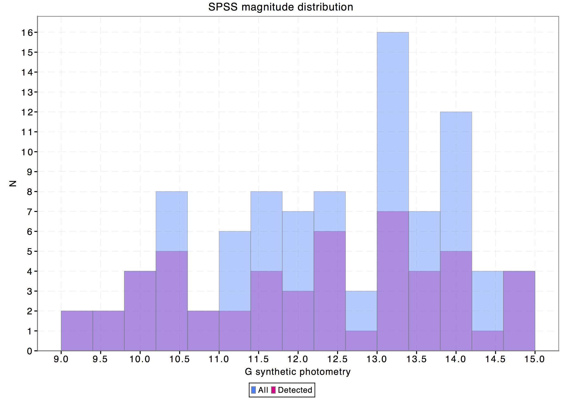
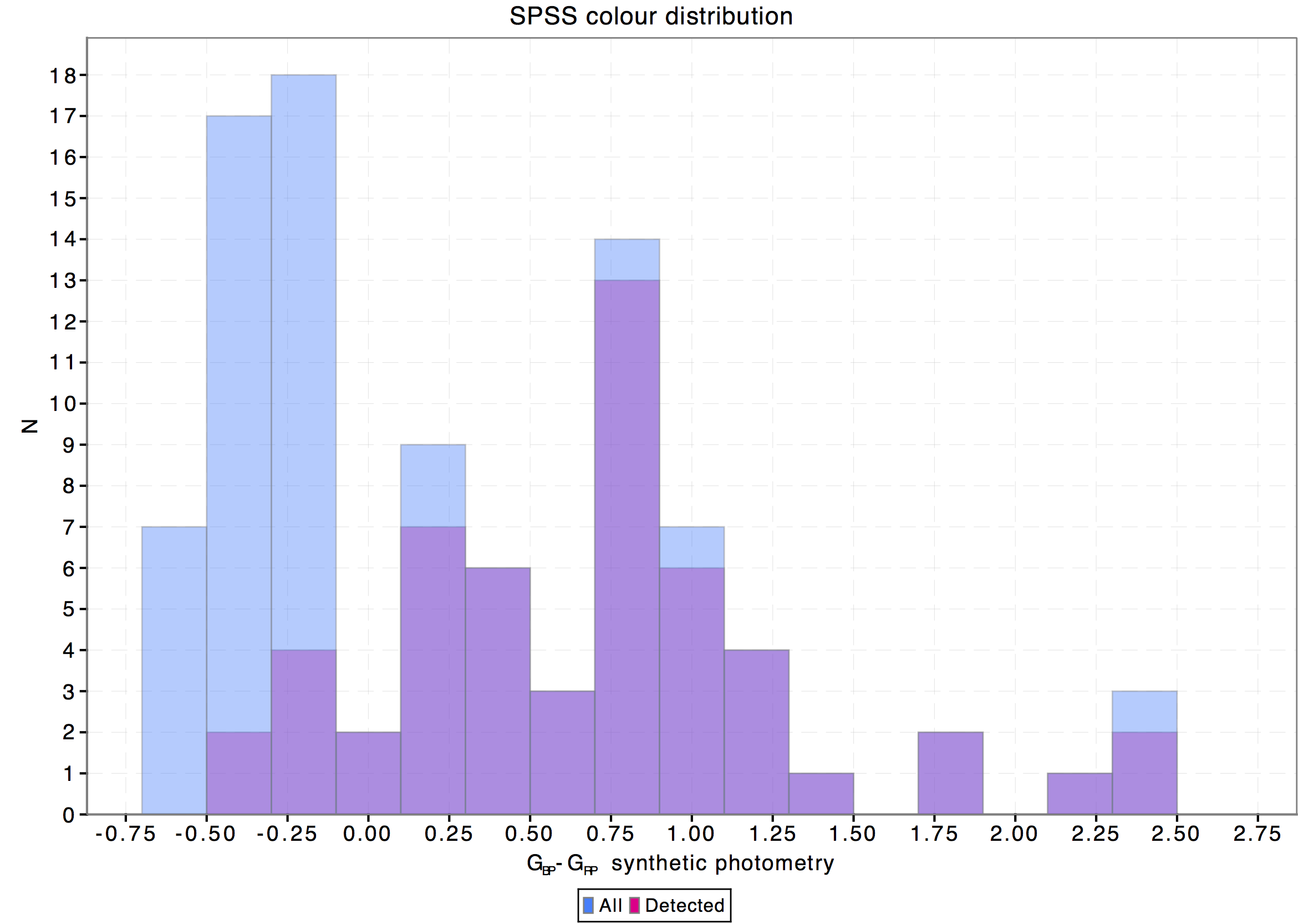
Figure 5.7: *Top*: Synthetic $G$ magnitude distribution of the SPSS exported by the internal calibration pipeline (purple histogram) against the corresponding distribution of the complete SPSS catalogue from the V1 release (blue histogram). *Bottom*: same data plotted against the synthetic $G_{\rm BP}$ $-$ $G_{\rm RP}$ colour.

To investigate the possible reasons for the rather large fraction of missing SPSS accumulated photometry we have checked the $G$ magnitude and $G_{\rm BP}$ $-$ $G_{\rm RP}$ colour distributions of the whole SPSS catalogue and the subset with available accumulated photometry. In both cases the magnitudes and colours have been derived through synthetic photometry on SPSS SEDs using the nominal pass bands (and hence nominal zero points). The resulting histograms are shown in Fig. 5.7: as can be seen most of the unexported SPSS lie in the colour range $G_{\rm BP}$ $-$ $G_{\rm RP}$ $<0.0$ . Further investigation made at DPCI pointed out that missing blue sources are due to a colour cut introduced by the time link calibration (TLC). The colour cut was determined by looking at the raw colour distribution of the 1000000 sources selected for the TLC: the selected range included the vast majority of the available data. Since the TLC uses Chebyshev polynomials, the colour cut was required to perform the normalisation and since the vast majority of the data was included, it did not seem worth to extend it any further. Future releases will remove this colour selection effect, making available the whole SPSS set.

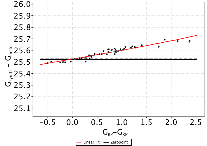
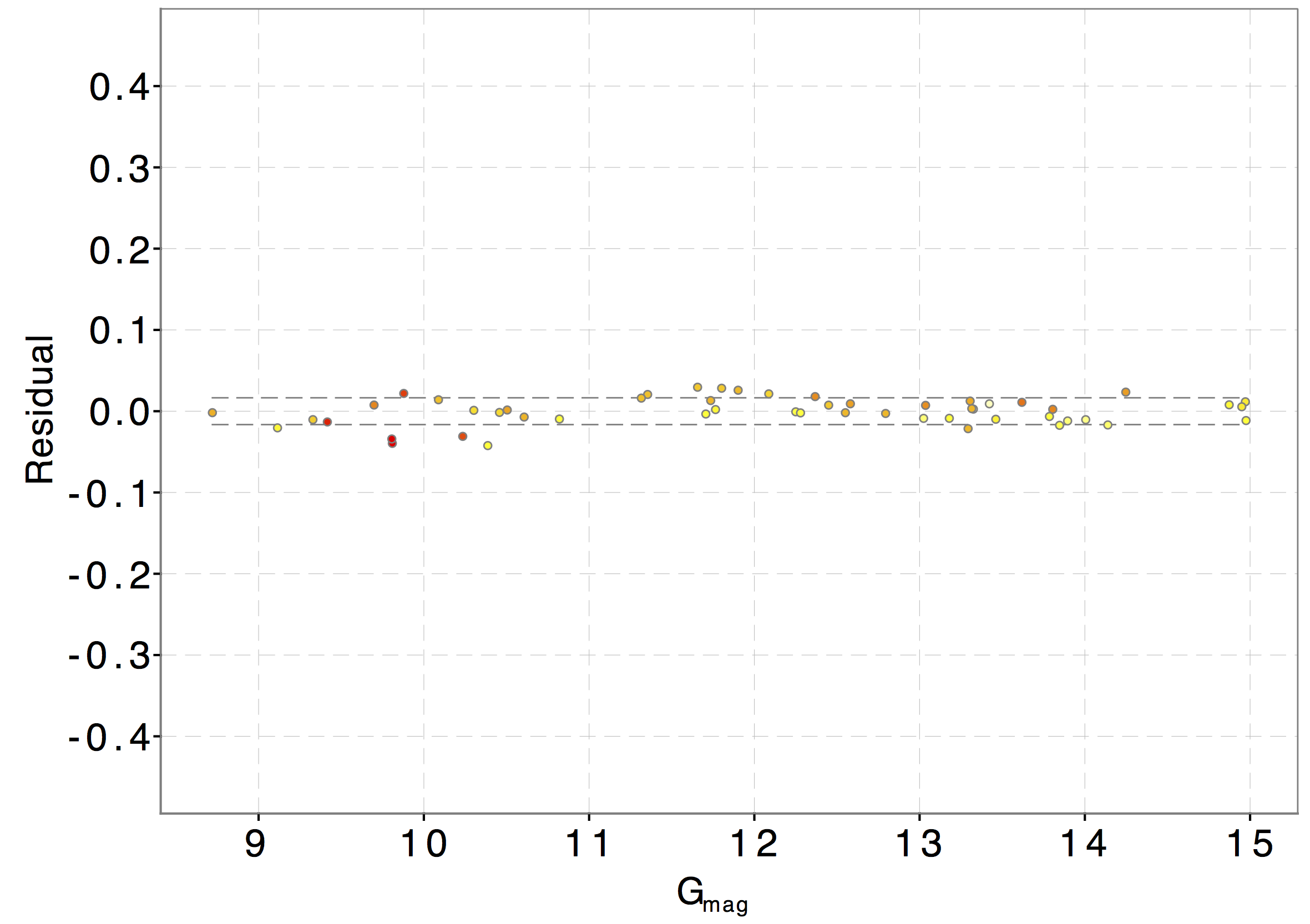
Figure 5.8: *Top*: $G$ band zero points $(G_{synt}-G_{instr})$ vs synthetic $G_{\rm BP}$ $-$ $G_{\rm RP}$ colours, showing the colour term due to nominal pass bands usage in the Gaia DR1 calibration. The solid black line represents the zero point corresponding to zero colour. The red line shows the least square fit of the colour equation. *Bottom*: Residuals $\Delta G$ with respect to the fitted colour equation plotted against the synthetic $G$ magnitudes: dashed lines represent the $\pm 1~{}\sigma$ level. The dot colours encode the $G_{\rm BP}$ $-$ $G_{\rm RP}$ colour of the sources (red dots showing reddest sources).

Fig. 5.8 shows for each SPSS the difference between the synthetic photometry in the $G$ band and the corresponding instrumental magnitude computed as 2.5 times the base 10 logarithm of the accumulated flux. These differences are plotted against the $G_{\rm BP}$ $-$ $G_{\rm RP}$ colour computed through synthetic photometry. The solid black line represents the derived external calibration zero point which results to be:

G_{0}=25.525\pm 0.003.

(5.26)

The external accuracy, estimated by comparison with some data catalogues (Hipparcos, Tycho-2, Johnson), is presently of the order of 0.01-0.02 mag (van Leeuwen et al. 2017), and is expected to improve in future data releases where the true pass bands (also for $G_{\rm BP}$ and $G_{\rm RP}$ ) will be used to derive the corresponding zero points.

To investigate for possible systematics left by the internal calibration we have computed the residuals with respect to a 1st order least squares fit of data displayed in Fig. 5.8 top panel (red line) and plotted them against the corresponding $G$ magnitude as shown in Fig. 5.8 bottom panel. As can be seen, no systematic effects are visible in the residuals.

A rough zero point was calculated also for the AB system, and is $25.696\pm 0.045$ mag (r.m.s. error), where the error is somewhat larger because the average value of $(G_{synt}-G_{instr})$ for all SPSS used.

5.3.5 Photometric relationships with other photometric systems

Author(s): Josep M. Carrasco, Holger Voss

This section includes some photometric transformations from $G$ to other common photometric systems (Hipparcos, Tycho-2, SDSS, Johnson-Cousins and Hubble systems are included here) using Gaia DR1 data with the zero point given in Eq. 5.26.

We crossmatched Gaia DR1 sources with those having available photometry in the external photometric systems to be considered. For Hipparcos and Tycho-2 relationships (see Sect. 5.3.5 and 5.3.5 respectively) we used TGAS Gaia DR1 data. For deriving relationships with SDSS photometry (Sect. 5.3.5) sources in SDSS data stripe 82 were used. Johnson-Cousins transformations (Sect. 5.3.5 were derived using Landolt stars. Finally sources of the M4 cluster were used to derive photometric transformations from Gaia to Hubble photometry (Sect. 5.3.5).

In order to obtain cleaner fittings, some filtering was done in each colour-colour diagram. These filters are indicated in Table 5.2 for every case. The polynomial coefficients obtained with the resulting sources are included in Table 5.3. The validity of these fittings is, of course, only applicable in the colour intervals used to do the fitting (see Table 5.4).

Table 5.2: Filters applied to fit the photometric relationships in Table 5.3 and the resulting number of sources considered for the fitting.

Tycho-2 filtering
$G-V_{T}=f(B_{T}-V_{T})$	$\sigma_{G}<0.01$ , $\sigma_{B_{T}}<0.05$ , $\sigma_{V_{T}}<0.05$
All Tycho-2 (335 305)	$G-V_{T}<0.5(B_{T}-V_{T})-2.1$
Blue range (130 467)	$B_{T}-V_{T}<0.9$ , $(\sigma_{\pi}/\pi)_{\rm TGAS}<0.1$ , $\pi>0$
Red giants (27 521)	$B_{T}-V_{T}\geq 0.9$ , $(\sigma_{\pi}/\pi)_{\rm TGAS}\leq 0.1$ , $\pi>0$ , $M_{G}\leq 4.0$
Red dwarfs (3109)	$B_{T}-V_{T}\geq 0.9$ , $(\sigma_{\pi}/\pi)_{\rm TGAS}\leq 0.1$ , $\pi>0$ , $M_{G}>4.0$
Hipparcos filtering
$G-H_{p}=f(B-V)$	$\sigma_{G}<0.01$ , $\sigma_{H_{p}}<0.1$ , $\sigma_{B-V}<0.1$
Blue range (48 766)	$B-V<0.8$ , $B-V\neq 0$
Red giants (14 759)	$B-V>0.8$ , $M_{G}<4.0$
Red giants (14 759)	$(\sigma_{\pi}/\pi)_{\rm TGAS}<0.1$ , $\pi>0$
Red dwarfs (2924)	$B-V>0.8$ , $M_{G}>4.0$ , $G-H_{p}<-1.3(B-V)+1$
Red dwarfs (2924)	$(\sigma_{\pi}/\pi)_{\rm TGAS}<0.1$ , $\pi>0$
$G-H_{p}=f(V-I)$	$\sigma_{G}<0.01$ , $\sigma_{H_{p}}<0.1$ , $V-I\neq 0$
(84042)	$-0.55(V-I)-0.2<G-H_{p}<-0.5(V-I)+0.2$
SDSS FILTERING
$G-g=f(g-i)$ (39 510)	$\sigma_{G}$ , $\sigma_{g}$ , $\sigma_{i}<0.01$
$G-g=f(g-r)$ (27 715)	$g-r<1.3$ , $\sigma_{G}$ , $\sigma_{g}$ , $\sigma_{r}<0.01$
$G-g=f(g-z)$ (36 199)	$\sigma_{G}$ , $\sigma_{g}$ , $\sigma_{z}<0.01$
$G-i=f(r-i)$ (42 846)	$\sigma_{G}$ , $\sigma_{r}$ , $\sigma_{i}<0.01$
JOHNSON-COUSINS FILTERING
$G-V=f(V-I)$ (336)	No filters
$G-V=f(V-R)$ and $G-V=f(B-V)$ diagrams
Blue range (273)	$V-I<0.14$
Red giants (34)	$V-I<0.14$ , $B-V\geq 0.6(V-I)+0.45$
Red dwarfs (37)	$V-I<0.14$ , $B-V<0.6(V-I)+0.45$
HUBBLE FILTERING
$G-F_{606W}=f(F_{606W}-F_{814W})$ (1165)	$\sigma_{G}<0.01$ , $G-F_{606W}>-0.35(F_{606W}-F_{814W})+0.05$

Notes. First column: diagram, followed in brackets by the number of sources. Second column: criteria applied

Table 5.3: Coefficients of the polynomials for sources observed in cycle 1.

Hipparcos relationships
		$B-V$	$(B-V)^{2}$	$(B-V)^{3}$	$\sigma$	Restrictions
$G-H_{p}$	0.0057225	-0.46999	-0.17444	0.14468	0.077	Blue range
$G-H_{p}$	-0.19891	-0.28654	0.086219	-0.11034	0.039	Red giants
$G-H_{p}$	1.6503	-5.458	4.9654	-1.6981	0.049	Red dwarfs
		$V-I$	$(V-I)^{2}$	$(V-I)^{3}$	$\sigma$
$G-H_{p}$	0.0029788	-0.54036	-0.0060301		0.041
TYCHO-2 RELATIONSHIPS
		$B_{T}-V_{T}$	$(B_{T}-V_{T})^{2}$	$(B_{T}-V_{T})^{3}$	$\sigma$
$G-V_{T}$	0.0079363	-0.4235	0.10048	-0.070742	0.066
		$B_{T}-V_{T}$	$(B_{T}-V_{T})^{2}$	$(B_{T}-V_{T})^{3}$	$\sigma$
$G-V_{T}$	0.049693	-0.62111	0.27735	-0.034246	0.057	Blue range
$G-V_{T}$	0.25566	-1.2049	0.83219	-0.27935	0.047	Red giants
$G-V_{T}$	0.44513	-1.5884	1.2706	-0.50446	0.063	Red dwarfs
SDSS RELATIONSHIPS
		$g-i$	$(g-i)^{2}$	$(g-i)^{3}$	$\sigma$
$G-g$	-0.098958	-0.6758	-0.043274	0.0039908	0.028
		$g-r$	$(g-r)^{2}$	$(g-r)^{3}$	$\sigma$
$G-g$	-0.081548	-0.96447	0.052098	-0.099175	0.027	$g-r<1.3$
		$g-z$			$\sigma$
$G-g$	-0.12166	-0.61201			0.035
		$r-i$	$(r-i)^{2}$	$(r-i)^{3}$	$\sigma$
$G-i$	-0.073784	1.2082	-0.82777	0.20293	0.028
JOHNSON-COUSINS RELATIONSHIPS
		$V-I$	$(V-I)^{2}$	$(V-I)^{3}$	$\sigma$
$G-V$	0.02266	-0.27125	-0.11207		0.028
		$V-R$	$(V-R)^{2}$	$(V-R)^{3}$	$\sigma$
$G-V$	-0.0076783	-0.35193	-0.7834	0.302	0.028	Blue sources
$G-V$	-0.41187	1.0915	-2.3259	0.68516	0.028	Red giants
$G-V$	-1.3918	4.8713	-6.5803	2.027	0.051	Red dwarfs
		$B-V$	$(B-V)^{2}$	$(B-V)^{3}$	$\sigma$
$G-V$	-0.034281	-0.084107	-0.46201	0.17151	0.045	Blue sources
$G-V$	-4.432	7.7846	-4.8557	0.88216	0.062	Red giants
$G-V$	-4.2544	9.6997	-7.1348	1.3729	0.121	Red dwarfs
HUBBLE RELATIONSHIPS
		$F_{606W}-F_{814W}$	$(F_{606W}-F_{814W})^{2}$	$(F_{606W}-F_{814W})^{3}$	$\sigma$
$G-F_{606W}$	0.13676	-0.48149	0.14654	-0.046247	0.036

Table 5.4: Range of applicability for the relationships found here between Gaia pass band and other photometric systems.

Hipparcos relationships
$G-H_{p}=f(B-V)$	Blue	$0.25<B-V<0.8$
	Red giants	$0.8<B-V<1.75$
	Red dwarfs	$0.8<B-V<1.6$
$G-H_{p}=f(V-I)$	Blue	$-0.2<V-I<3.5$
TYCHO-2 RELATIONSHIPS
$G-V_{T}=f(B_{T}-V_{T})$	All range	$-0.2<B_{T}-V_{T}<2.0$
	Blue	$-0.15<B_{T}-V_{T}<0.9$
	Red giants	$0.9<B_{T}-V_{T}<2.25$
	Red dwarfs	$0.9<B_{T}-V_{T}<1.75$
SDSS RELATIONSHIPS
$G-g=f(g-i)$		$-0.4<g-i<3.0$
$G-g=f(g-r)$		$-0.3<g-i<1.3$
$G-g=f(g-z)$		$-0.3<g-i<4.3$
$G-i=f(r-i)$		$-0.2<g-i<1.6$
JOHNSON-COUSINS RELATIONSHIPS
$G-V=f(V-I)$		$-0.25<V-I<3.25$
$G-V=f(V-R)$	Blue	$-0.2<V-R<0.8$
	Red (giants & dwarfs)	$0.7<V-R<1.4$
$G-V=f(B-V)$	Blue	$-0.2<B-V<1.25$
	Red giants	$1.25<B-V<2.3$
	Red dwarfs	$1.25<B-V<1.8$
HUBBLE RELATIONSHIPS
$G-F_{606W}=f(F_{606W}-F_{814W})$		$0.45<F_{606W}-F_{814W}<1.5$

Hipparcos relationships

Photometric relationships between Gaia and Hipparcos are obtained here by using TGAS data.

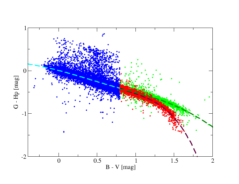
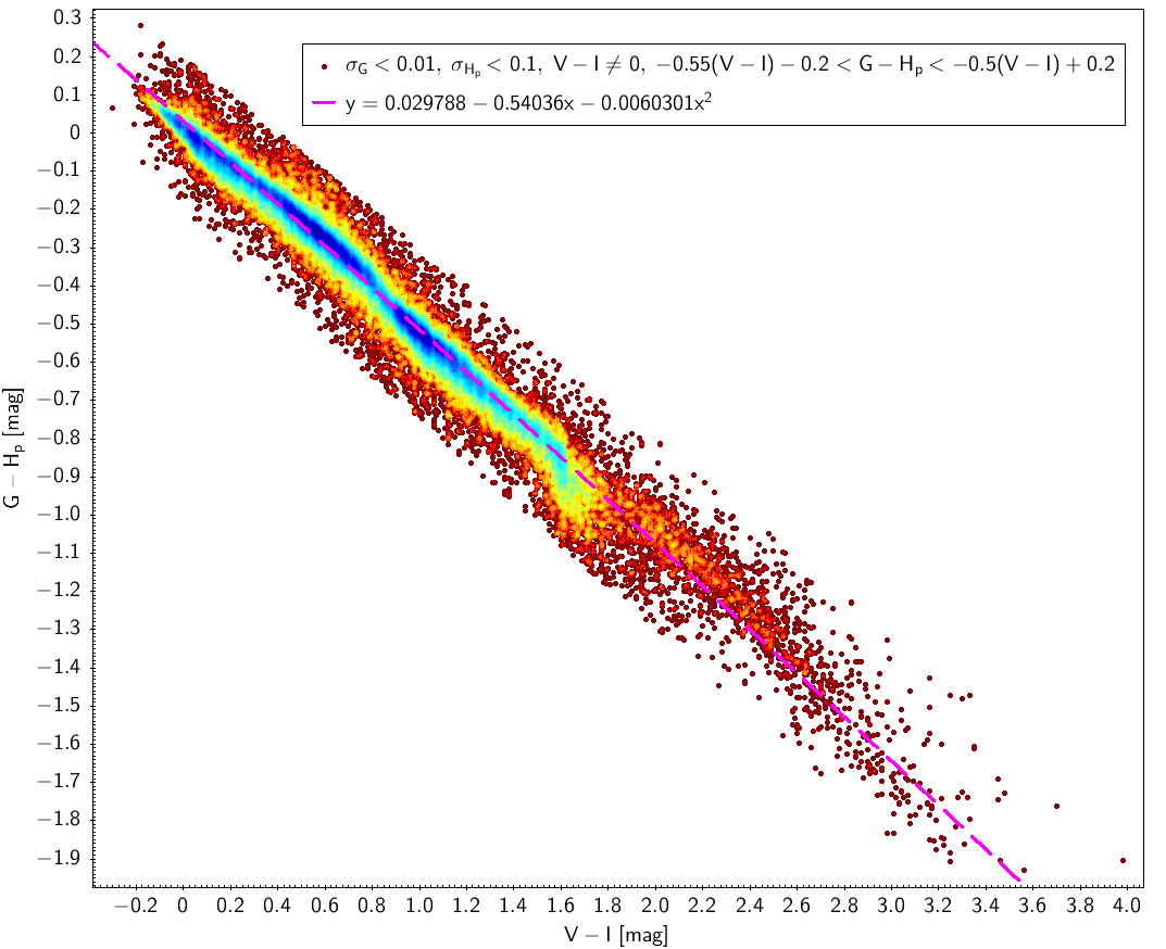
Three different laws for $G-H_{p}=f(B-V)$ were fitted: one at the blue range and two at the red range (one for giants and another for dwarfs), see Fig. 5.9 (left panel). Absolute $G$ magnitudes were derived using TGAS parallaxes ( $M_{G}=G+5\{1+\log[\pi(mas)/1000]\}$ ). $M_{G}=4.0$ mag is the used threshold to separate giants and dwarfs for $B-V>0.8$ .

Figure 5.9 (right) shows the fitting for the $G-H_{p}=f(V-I)$ case (no giant and dwarf distinction was needed in this case as both types of sources share the same behaviour in this diagram). In order to allow a better behaviour outside the fitted interval we reduced the degree of the polynomial to second order.

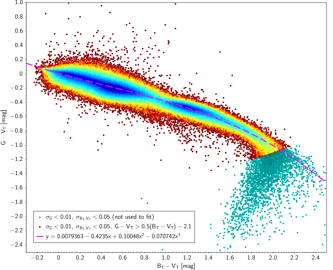
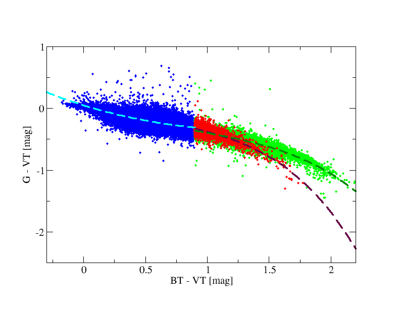
Figure 5.9: Fitting of $G-H=f(B-V)$ (left) and $G-H=f(V-I)$ (right) relationships obtained for Hipparcos data.

Tycho-2 relationships

The TGAS data set is used here to derive the relationships between Gaia and Tycho-2 photometry. A starting set of 1 962 085 TGAS sources (before filtering as given in Table 5.2) was cross matched with Tycho-2 catalogue based on their coordinates.

Figure 5.10 (left) shows the fitting obtained using only Tycho-2 information. Analogously to Sect. 5.3.5 we split the fitting again in red giants and red dwarfs ( $M_{G}=4.0$ mag is also used to separate giants and dwarfs) using TGAS parallaxes (Fig. 5.10, right), although the result is not so clean in this diagram as in the Hipparcos case.

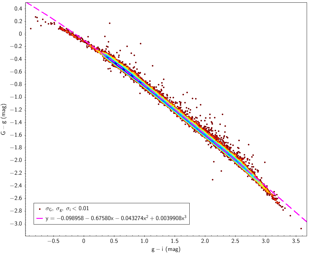
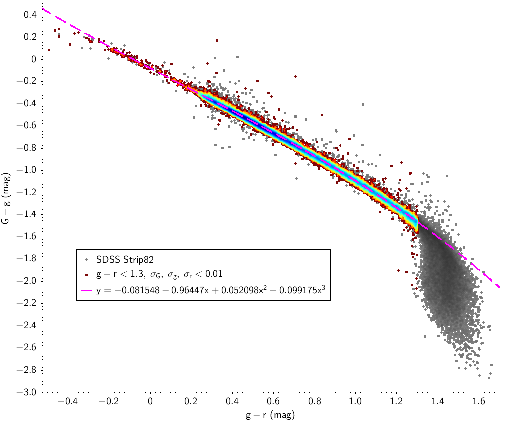
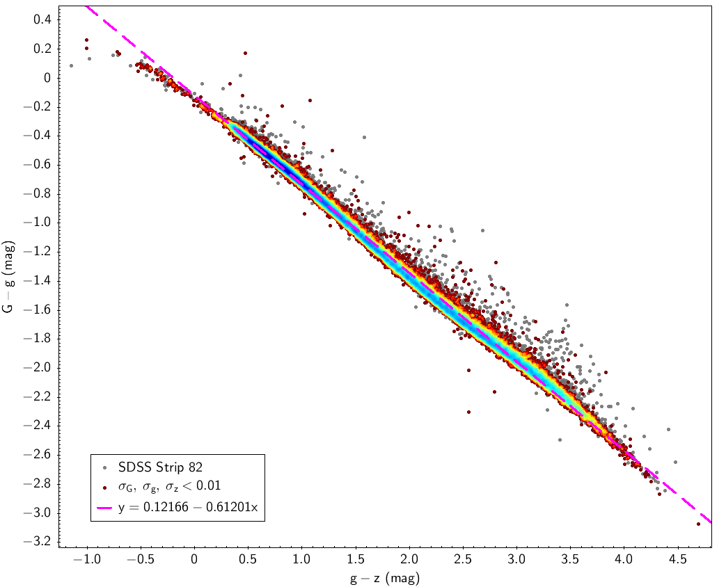
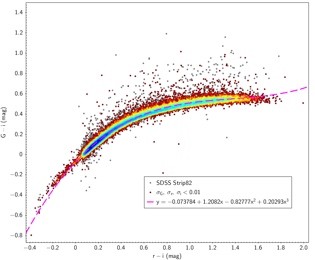
Figure 5.10: Photometry fitting obtained for $G-V_{T}=f(B_{T}-V_{T})$ relationship obtained for all available Tycho-2 data (left panel). The right panel shows the same diagram when trying to use TGAS parallaxes as discriminator between dwarfs and giants with $B_{T}-V_{T}>0.8$ . .

SDSS relationships

SDSS stripe 82 data is used here with the filters indicated in Table 5.2 for SDSS sources. Table 5.3 and Fig. 5.11 show the fitting laws obtained using this data.

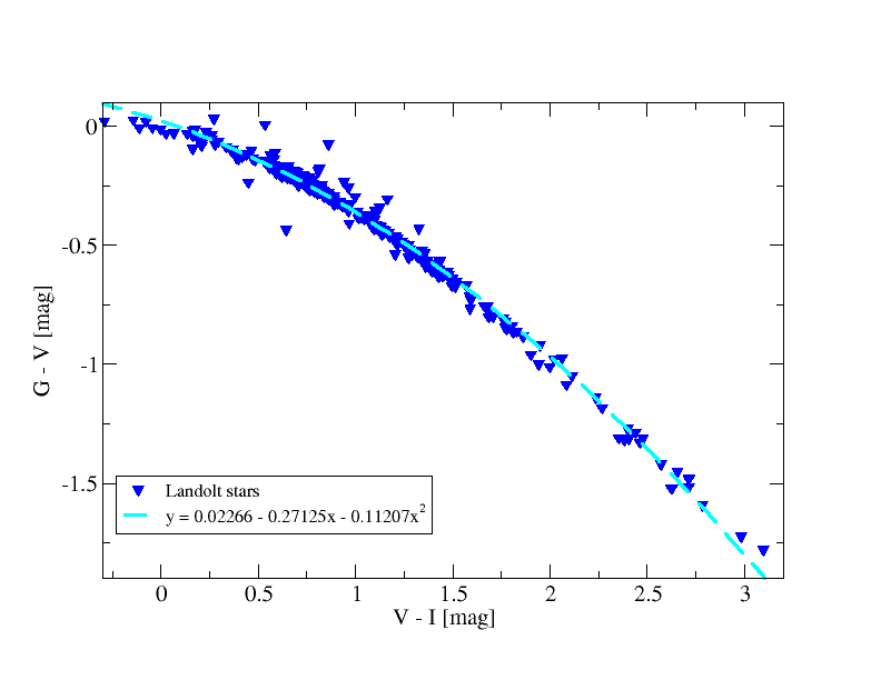
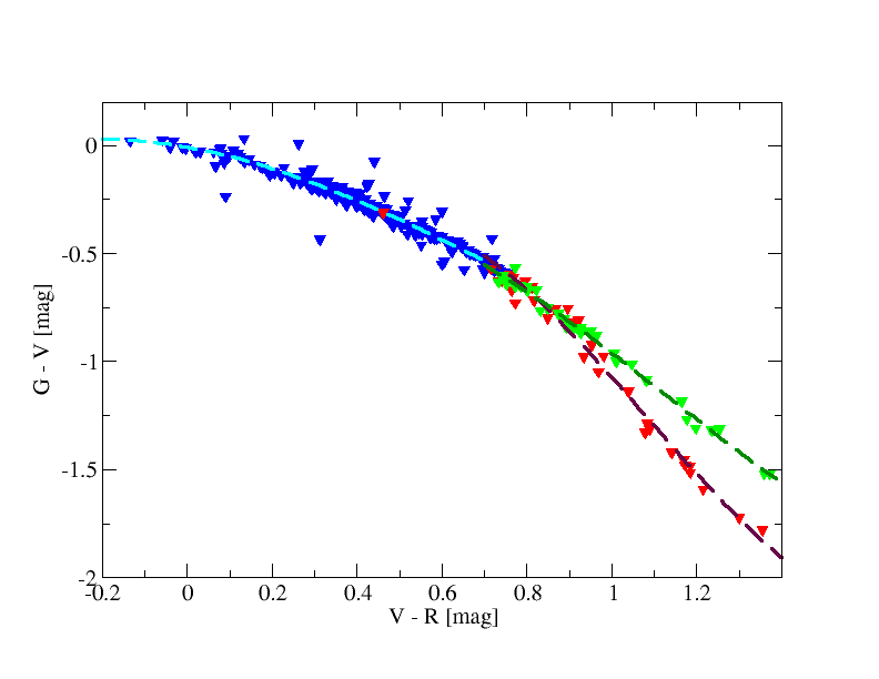
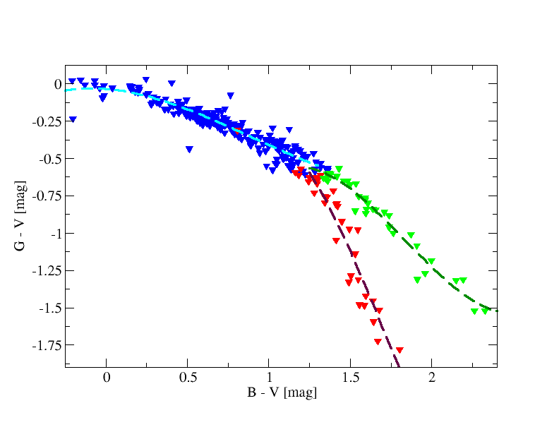
Figure 5.11: The left panel shows the selection done to produce the fitting shown in the right panel for SDSS stripe 82 stars processed in PhotPipe cycle 1.

Johnson-Cousins relationships

We used Landolt stars observed by Gaia to get transformations between Johnson and Gaia (see Fig. 5.12). For the red stars we split the fitting in dwarfs and giants based on $B-V=f(V-I)$ diagram (see Table 5.2).

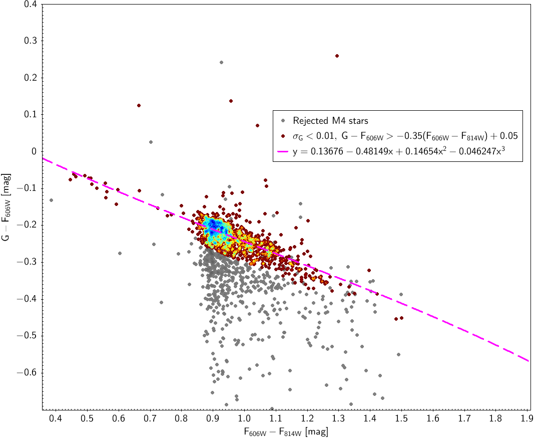
Hubble relationships

Using sources of the M4 cluster (NGC6121) in Gaia DR1 crossmatched with the corresponding stars with Hubble photometry ( $F_{606W}$ and $F_{814W}$ pass bands in Vega system) we derived transformations between the two photometric systems. Figure 5.13 shows the obtained fitted laws.

European Space Agency

Science & Technology